IEC 60601-2-2 Calculator for HF insulation testing (201.8.8.3.102, 201.8.8.3.103)

While bench testing is often used as the formal evidence of compliance, it is best when paired with design calculations that show a specification can be reliably met with suitable margins, independent of the bench test. The calculator below is intended for use with IEC 60601-2-2 Clauses 201.8.8.3.102 (HF leakage current) and 201.8.8.3.103 (HF dielectric strength). The calculator uses two insulation material properties (relative permittivity, dissipation factor) and three design specifications (insulation thickness, wire or shaft diameter, rated peak voltage) as well as the sample length to estimate capacitance,
HF leakage, HF dielectric strength test parameters, currents and loads, sample heating and temperature rise.

Parameter	Value	Units	Description/Notes
Insulation thickness: (symbol d)		mm	Insulation thickness on the wiring or shaft (for example, the recovered wall thickness for heatshrink). Typical values are between 0.1 and 0.5mm. HF leakage is inversely proportional to thickness, and dielectric heating is inversely proportional to thickness squared
Relative permittivity: (symbol ε)		(unitless)	"Permittivity" relative a vacuum, typical values for insulation are 2.0 to 3.0. Materials with high values such as PVDF (over 8.0) are not recommended as these will have high leakage currents and dielectric heating.
Dissipation Factor (DF): (symbol δ)		(unitless)	This is the proportion of the apparent power (VA) that gets turned into heat, in effect the resistive part of the insulation. This parameter has a major effect on dielectric heating. In specification sheets this may be expressed as a percentage (e.g. 2% == 0.02) or as "x10-4" (e.g. 200 == 0.02). It is generally recommended to use materials with DF ≤ 0.001 especially for insulation thickness ≤0.3mm.
Shaft or wire diameter: (symbol D)		mm	This is the diameter of the metal part, excluding the insulation thickness. For wiring this would normally be around 0.3-1.0mm, for shafts typically 3-8mm
Length to analyse: (symbol L)		cm	This is length in cm to be analysed for total capacitance and loading effects only. Other effects are density based and so the length it not relevant. This is important to consider the loading on the test equipment and ESU
Rated voltage: (symbol Vr)		Vpeak	This is the rated peak voltage which will be disclosed in the instructions for use. It is used to calculate the test voltage (120%) and test Vrms, expected currents and heating. Note that it should not be confused with Vpp (peak to peak) which is sometimes used for generators.

CALCULATE

Capacitance density: Symbol Ca		pF/cm²	Capacitance per unit area, usually in the order of 5-15pF/cm². For compliance with IEC 60601-2-2 this is the most important factor, as effects are density related. High values of capacitance leads to high loading, HF leakage currents and dielectric heating (lower is better) Using C=0.8854ε/d, based on C = ε0εrA/d (F)
Capacitance of sample: Symbol Cs		pF	Sample capacitance (or capacitance of length L), which is important for loading of test equipment and also the HF generator (ESU). Using C = 0.278 εr L (D+d) /d, based on C = ε0εrA/d (F) Notes: *The MEDTEQ HFIT 8.0 is designed for 150pF up to 6kVp and 100pF for 7.2kVp. If necesary shorten to a representative sample length *Excessive sample capacitance can also overload HF generators (ESUs) *This formula uses an approximation of the cylinder capacitor unwrapped into a parallel plate capacitor. A more precise method is C = 2πL/ln(r2/r1)
HF Leakage (per unit area) (@400Vp 400kHz)		mA/cm² (Limit 10mA/cm²)	This estimates the HF leakage current per cm², using Ca, for a sine wave test voltage of 283Vrms (400Vp) at 400kHz. Using I = 0.7018Ca, based on I = 2πfVC (A) As explained in IEC 60601-2-2 rational, original limit is based on 25mA/cm² @ 800Vpp (283Vrms = 400W for 200Ω), 1MHz. This is adjusted to 10mA/cm² for a typical test frequency of 400kHz. Although not specified in the clause, by definition leakage currents are always based on rms values.
HF Leakage (sample) (@400Vp, 400kHz)		mA Limit: mA	This estimates the HF leakage using Cs instead of Ca. In actual tests the measurement will depend on the actual lengths, frequency, voltage, however the limit will also be adjusted proportionally. The actual measured results should be similar region. The limit is based on 10mA/cm² and using the sample surface area using the length above and diameter based on the wire/shaft plus two times the insulation thickness (D+2d).
HF Dielectric Strength Test voltage, peak		Vp	The test voltage in IEC 60601-2-2 is 120% of the rated voltage
HF Dielectric Strength Crest factor target (CF)		(unitless)	For Vr ≤1600Vp, CF ≤2 (for the calculation a sine wave is assumed CF = 1.414). For Vr = 1600-4000V, the CF is determined from the formula CF = (Vr - 400)/600 For Vr≥ 4000, CF is 6.0
HF Dielectric Strength Vrms		Target Vrms	Calculated using Vrms = 1.2 * Vr / CF
Sample impedance		jΩ	Impedance of the test sample at 400kHz (length L), using Xc = 1/(2πfCs)
HF Dielectric Strength Peak current		A (peak)	This is based on the peak voltage and impedance Xc. This is indicative of the currents that may load an ESU in clinical applications.
HF Dielectric Strength Peak power	[]	VA [kVA!!!]	Based on the peak voltage and peak current above, indicates the peak power the test equipment needs to supply to reach the peak voltage.
HF Dielectric Strength rms current		Arms	This is based on the rms voltage and impedance of the test sample Xc.
HF Dielectric Strength rms load		VA (rms)	This is the rms (average) VA load to the test equipment and also on which dielectric heating is based.
HF Dielectric Strength Heat		W (Watts)	Based on the dissipation factor, this is the amount of actual heat in the test sample (for length L)
Dielectric heating, Temperature rise after 30s		°C (or K)	This is the estimated temperature rise based on the heat above, a volume of π(D+d)Ld, a heat capacity of 1.5J/K/cm³ (typical), and a test time of 30s. This estimate assumes no heat is lost, but in practice there will be heat absorbed by the shaft/wire, conductors/liquids/cloth in contact with the insulation surface, convection and radiation. Even so it provides a good indicator for dielectric heating. It is recommend to use materials with <10K rise by this method.

Li-ion batteries - the anecdotal PCM story

If you are new to Li-ion batteries and standards compliance in the context of IEC 60601-1, the area can be confusing - largely because there is some messy history. Normally with a high risk part such as this you can buy it off the shelf, all nicely certified, well specified, just plug and play.

To a large extent battery manufacturers have done their job well, especially if you are dealing a reasonably well known, quality battery maker. The weak point is mostly on the standards and third party testing. It is improving, and perhaps in a few years an article like this will no longer be needed.

OK, before we start some basic terms.

Standards refer to “primary” and “secondary” cells or batteries - translated this means “non-rechargeable” and “re-chargeable” respectively.

Standards also refer to “cell” and “battery”. Normally lay people mix up battery and cells, while us experts know that “battery” means two or more cells. Well, forget that. For IEC standards, a “battery” means one or more cells together with any necessary protective features. Any sizable cell will normally have a PCM or Protection Circuit Module, so even a single cell with a PCM is referred to as a “battery”.

This article is intended for a re-chargeable cells with a size large enough to need a PCM, i.e. secondary batteries. Anecdotally, the threshold for this seems to be around 50mAh, although no literature has been found to support this. This article, by the way, is all anecdotal - please use it to power your own research, but not as a resource itself.

Now for some basics on Li-ion safety.

Li-ion is generally safe compared to the original lithium metal batteries. However, under overload, short, overcharging and age, the Li-ion can convert to metal and become highly flammable. In order to protect against this, most cells will have three protection features inside the cell, including a PTC for overcurrent, a pressure switch for overcharging (triggered by gas production), and finally a vent (weak point) to release pressure in case the other two fail.

But … these protection features are not what we would call super reliable. They might work, say, 19 out of 20 times. I have no idea of the actual value, only that it’s nowhere near the normal reliability we would expect for a safety feature associated with fire.

Thus, once the cell gets to a certain size, say >50mAh, most manufacturers will fit a PCM. This is a small electronic circuit that watches the cell voltage, charge and discharge currents and disconnects the battery if anything exceeds the limits. It’s usually built into the pack, a small PCB at the top which can sometimes be seen if the final wrap is clear. There are many dedicated ICs that can perform this function with just a few external components, and there are ICs for multi-cell packs that can watch each cell individually. The PCB also often contains a 10k NTC thermistor - more on that later.

This “battery”, which contains cell(s) with protective features (PTC , PS, PV) plus the PCM is what you will typically find on the market today. As long as the end product manufacturer makes sure the charging circuit fits within the normal condition limits as specified by the battery manufacturer (currents, voltages, profiles, temps) then the overall system is safe in normal and single fault condition. Plug and play.

So far so good. But in the modern world, for high risk things like preventing fire it is not enough to trust a spec sheet: it has to be verified in design and production, with regulatory records. To avoid that every end user has to audit the battery manufacturer, we normally rely on third party certification.

This is where things fall off the rails.

Third parties are generally good at all the cell side of things - cells normally have a bunch of stress tests thrown at them to show they are unlikely to explode or catch on fire. However, for larger cells the charging voltage is normally limited during testing to the values specified by the manufacturer, for example 4.35V for a typical 3.7V cell.

Why?

My guess - historically, UL were the market leader, UL1642 certified cells were (are?) the defacto standard. Knowing that larger cells can occasionally explode if overcharged, their approach was to test to the limits specified by the manufacturer (e.g. 4.35V) and then “list” the cells using these limits, requiring that the end user would ensure these limits are not exceeded in normal and single fault condition.

End product manufacturers however, not being aware of the dangers, often missed the “single fault condition” part and designed chargers around normal condition only, typically 4.25V. In fact, the only way to cover the single fault condition successfully is to have a fully independent circuit between the charger and the battery, something that is not intuitive for an end product designer. Moreover, in the case of a series of cells (e.g. 7.2V, 14.8V packs) it is not possible to monitor the individual cell voltage external to the pack, so UL’s approach was actually an impossible to meet.

Battery manufacturers knew this, and started fitting PCMs to packs to handle the single fault condition. It’s perhaps a rare case where manufacturers got ahead of the agencies, which in turn clearly indicates that Li-ion is definitely dangerous stuff. If it was all just theoretical, there is no way the PCMs would be fitted unless pushed by the agencies.

It’s also possible that agencies knew about the importance of PCMs but were reluctant to accept electronic based protection: historically “protection” is in the form of fuses, circuit breakers, optocouplers, insulation, earthing, where the protection itself can be tested for various aspects reliability. Electronic circuits don’t lend themselves to this kind of verification. In the real world though, the PCM is a very simple circuit and modern electronics is generally reliable - like 10-9 events per year kind of realm - in practice a PCM is far more reliable than a fuse or circuit breaker.

That of course is history, and standards and third parties are catching up. The latest standard IEC 62133-2:2017, which is dedicated for re-chargeable Li-ion cells and batteries, does allow for testing that includes the PCM.

However this standard was only released in 2017, so much of the documentation on Li-ion batteries may pre-date this. The older standard IEC 62133 does not reliably test the PCM, nor does UL1642 or UL2054 listings.

Confusingly, IEC 62133-2 can be used for both cells and batteries. If the report is just for the cells it won’t cover the PCM and various other tests. By using the same standard number for cells and batteries means that users need to look into the report to figure out what is going on. I guess that in the future we may see a new standard covering a “battery pack”, to mean an object that has all the protective features built in, that the end user can really just plug and play.

A side issue is that battery packs are often custom designed, and there are a wide range of sizes and shapes available, some are fairly specialized and low volume. Forcing manufacturers into third party certified pack route may not be feasible. Thus a real long term solution may also see a consolidation and standardization of the available pack size, ratings, and physical shape, which itself may not be a bad thing.

OK, with all that in mind, how to deal with Li-ion batteries and IEC 60601-1?

For secondary batteries, IEC 60601-1/A1:2012 Clause 15.4.3.4 refers to an compliance with IEC 62133. Since this is undated, technically the latest edition should be used, which is IEC 62133-2:2017. It’s also important to note that the standard refers to “secondary batteries” not “secondary cells”, which in turn means that the PCM, if required for safety, must be included in the testing.

Note that if you are reading the earlier version of IEC 60601-1:2005, it has an incorrect reference to IEC 60086-4 which is only for primary or non-rechargeable batteries. This was corrected in A1:2012.

When you ask battery manufacturers for evidence of compliance they may provide a few different things:

Some may provide reports for the old IEC 62133:2012. This standard may be OK for the cell, but it may not cover the PCM.

Some manufacturers may point to UL1642 listing. This is an older standard, and not IEC aligned, but is reasonably seen as equivalent to IEC 62133. However, it again it is just for the cell and does not cover the PCM.

If you are lucky, the manufacturer might provide a report for IEC 62133-2:2017 which is the the newer version and covers the PCM. However, you need to check the report (not just for example, the CB certificate) to make sure it is for the battery pack and not just the cells. Also reports (and CB Certificates), only cover the samples tested, and don’t cover regular production. Legally, you need to be covered for design and production. As such, even if you have a report, it’s recommended to ask for a declaration of conformity, since a properly prepared declaration covers both design and regular production. Make sure the declaration refers to IEC 62133-2:2017 (dated), and make sure it covers the pack with the PCM, not just the cells.

If you are really lucky you might get:

• UL listing to UL62133-2:2020. This UL standard is fully harmonized with IEC 62133-2:2017 and covers the PCM, and if the part is UL listed this means it includes a factory inspection (i.e. production is covered)

• any other private certification marks such as TUV SUD, TUV Rh, VDE etc, which has the latest standard (IEC 62133-2:2017) and includes factory inspection.

These last two are truly plug and play. However, it is expect these will take a while to get popular.

In the mean time, what to do if really like the pack but the evidence is weak and may not cover the PCM?

The first point is to check if a PCM is fitted. This is usually indicated in the specification sheet.

Next, there are a few options, which could be taken in combination:

1. Trust the manufacturer: if it is a well known brand this might be enough for some users

2. Ask the manufacturer for a declaration of conformity to IEC 62133-2:2017 covering the battery pack with the PCM installed (as above)

3. Periodically inspect and test packs for implementation and correct operation of the PCM. Note this needs to be done in a safe way considering the risks of exploding batteries.

If there is no PCM or the implementation cannot be confirmed, it’s also possible to fit your own PCM external to the pack, provided that it is single cell only.

If the cell is small enough that a PCM is not required, note that this still needs evidence. The cell certification should be compatible with the voltage/current available in fault condition from the end product. For example, if the charging IC is run off a 5V/500mA USB supply, then if the charging IC fails, these would be the most expected in fault condition. If you have say UL1642 cells certified to 5V/1A, then that might be enough.

Apart from above, from experience end product manufacturers sometimes mess up the charging characteristics. Most charging ICs are flexible and there are several parameters which can be set by external components. It’s always worth having an independent engineer double check the calculations. Wireless chargers have extra complexity and worth to double check the charging parameters and profile is as expected.

In 2007 the Japanese organisation JEITA issued a guideline on temperature limitations for Li-ion charging. Many chargers now work with these limits, using an NTC that is situated close to or inside the pack. It is recommended to use this feature if possible to maintain battery life and for additional safety (less chance of the other protective features being activated). Many packs have a third lead with a 10k NTC fitted for this purpose.

These last two points are technically covered by IEC 60601-1 Clause 4.8, which requires that components are used within specification. However, not all test agencies will check the detail, so it’s worth double checking internally with an independent engineer.

In addition to IEC 60601-1, most people would have heard of UN 38.3 which covers shipping. I’m not an expert on this, but I assume a declaration might be needed before agencies like DHL, FedEx, UPS etc will accept batteries for shipping.

There is also an EU battery directive. Again it is not an area of expertise but from memory there is a requirement to provide a practical method for removing the batteries for disposal. In other words, simply saying “dispose of according to national regulations” in the IFU may not be enough.

A final reminder! All information here is provided to help designers get started, but should not be used as a formal reference. Always check the source regulations, standard etc for the final decision, and if necessary engage qualified experts.

ECG Low Frequency Response Impulse test (0.05Hz, 3mV/100ms test)

Recently Derek Qin of Draeger pointed out that at the end of the MEDTEQ article on ECG filters, the graph showing the effect of a 3mV/100ms impulse on a 0.05Hz high pass filter had a post impulse slope that looked more like 29µV rather than the claimed 291µV.

It turns that Derek was right, the correct answer is 29µV/s, but there’s actually a lot more to the story of this apparently simple test.

The mistake, by the way, escaped through the usual checking process of calculation by two different methods: first by excel step-wise simulation and the next with simple math for exponential decay and the derivative. Both had different errors, and by chance both errors arrived at ~291µV/s.

But perhaps it was more than a rare double mistake. Compared to actual test results, 29µV/s is far too low. And why have a limit of 300µV/s if the practical result is <10%. So it’s likely that bias played a role. In fact, when tackling this issue 10 years later, the author was convinced it was 29, and then reverted to 291, before finally settling back to 29. And this still did nothing to explain the difference with real world test results or why the limit is so high.

After throwing around a few ideas, Derek again came to the rescue by pointing out that my original calculations were based on a single, uni-polar pulse in isolation. In the case of a series of pulses (pulse train), the results can be widely different due to the waveform shifting down to accommodate the dc offset, which then dramatically increases the absolute value of the overshoot, relative to the dc level. This in turn increases the slope of the decay. This can be best seen by looking closely at the following image:

View fullsize

A pulse train of 3mV/100ms impulses repeated at 0.5Hz (30bpm), expanded to see the effect around the baseline. The slope of the last pulse is clearly different to the slope of the first pulse

(click on the image to expand)

It turns out that in the case of a pulse train, the results will depend on:

(a) The pulse frequency (pulse repetition rate)

(b) The time the test is run (which pulse in the sequence), and

(c) The simulator’s offset

Clearly, this is not intuitive, so let’s run through the math starting off again with a single unipolar 3mV/100ms pulse (for those not interested in the math, jump to the conclusion):

Overshoot: The initial 3mV positive edge passes through the high pass filter without distortion, and then starts to decay based on the time constant τ = 2πf = 3.18s. The decay after 100ms is D = A(1- exp(-t/τ)) = 3mV x (1- exp(-0.1/3.18)) = 0.093mV = 93µV. The 3mV negative edge at the end of the pulse also passes through the filter. Since the waveform has decayed 93µV, this decay value appears directly as an overshoot.

Slope: The slope is then calculated from the derivative of the exponential decay, using the overshoot as the starting amplitude A:
S = -A/τ = - -92.87µV / 3.183s = +29µV/s

Now let’s take a look at a pulse train, first using 1Hz frequency (60bpm), which has been allowed to “settle”. A 0.05Hz filter has a time constant of 3.18s, so it takes about 15s to 20s to stabilise after any shift in dc offset (15s = 1% error, 20s =0.2% error). A 3mV/100ms pulse repeated at 1Hz has an initial dc offset of 0.3mV and will eventually settle to a waveform with maximum +2.7mV and minimum -0.3mV relative to the dc level. We can then re-calculate using the above method, but with these settled values:

Overshoot: D = A (1- exp(-t/τ)) = 2.7mV x (1-exp(-0.1/3.18)) = 0.0825mV = 83.5µV

Slope: The new slope is calculated based on the overshoot and the -0.3mV (-300µV) offset that is the minimum of the settled waveform. Thus,
S = -A/τ = - (-300-83.5)µV / 3.183s = +121µV/s.

We can see here that the overshoot is only mildly affected, but the slope is wildly different. This explains why practical results are very different to 29µV/s predicted from a single pulse.

The result is obviously affected by the pulse frequency since this influences the max/min values of the settled waveform. For example, a 0.5Hz (30bpm) pulse train will settle to +2.85 / -0.15mV, and 2Hz (120bpm) waveform settles to 2.4 / -0.6mV.

And … if the waveform is not settled, it depends on which pulse is used. An engineer might run the test and randomly pick the 5th pulse, and later run the test again and pick the 12th pulse, and scratch their head as to why the results are different. So the test should be allowed 20s to settle in order to guarantee consistent results.

But that’s not all. It’s possible that the ECG simulator could use a -50% offset which can effectively double the range of the simulator for pulse waveforms (as used in the SECG). Instead of making a pulse using 3mV/100ms and then 0mV for 900ms, the simulator could use +1.5mV/100ms, -1.5mV/900ms. While the waveform is settling, this initial offset can dramatically influence the result, and can even exceed the 300µV/s limit for the first few pulses. Again, if the test is allowed to run for 20s this effect is eliminated.

This all explains a lot. And it turns out this issue affects any ECG testing where there is a dc offset in the test waveform and the ECGs filter goes down to 0.05Hz. Examples are such as the 200/20ms test and the CAL20160 waveform. More work is required to simulate these waveforms and determine the extent of the impact, but in the mean time, it makes sense to allow these tests 20s to stabilise and fix the test frequency.

Conclusion

Based on the above analysis, all tests involving a 0.05Hz filter should be:

• allowed 20s to stabilise

• be tested at 1Hz if not specified, or at least with the test frequency included in the test record to allow the test to be repeated

Ideally, future versions of ECG standards should include both the stabilisation time and test frequency for all tests.

If there are still errors in the above analysis, please feel free to report them.

Medical systems - a device based approach

This article covers the handling of medical devices that are intended for use in a larger system, where other parts of the system are placed on the market independently, such as a patient monitors that is designed for used with accessories from another manufacturer.

It is provided in pdf format to allow printing for the long read.

MQ001 Medical Systems - A device based approach (pdf)

ECG - input impedance and noise

In ECG standards, clauses such as 201.5.3 cc) of IEC 60601-2-25 require that test signals are accurate to ±1%. Although not explicitly stated in the standard, it’s obvious that this includes noise. If for example a test requires the ECG under test to reproduce a test signal accurately within ±5%, it would make no sense to perform the test if the test signal also had say ±20% noise.

Some engineers however might consider environmental (common mode) noise as a separate issue. ECGs are required to work in noisy environments so they should have the ability to reject common mode noise. Hence testing in a normal “noisy” environment is representative of the real world. This is wrong for two related reasons: first the ECG is anyhow tested for the ability to reject noise including common mode noise; second is that in order to test objectively, we need to start with a low noise environment and then add test signals including noise in a known and accurate way.

As such, while there are no instructions, notes, requirements or methods in the standard to minimise noise, such actions are implicit in the requirement to apply test signals with an accuracy of ±1%. In particular, most test signals are in the order of 1mV, which means noise of just 10µV is significant. Normal methods to minimise noise include using a ground plane under the ECG, cables and test equipment, and connecting the ECG equipment earth (PE or FE) and the test circuit ground to the ground plate.

The input impedance test is by far the most sensitive to noise, and sometimes the normal procedures are not enough. The reason for the high sensitivity to noise is the large imbalance impedance. To understand why this is so, it is useful to review the article on CMRR testing, which explains how CMRR is really a function of leakage currents flowing through the imbalance impedance. It follows that the size of the imbalance impedance directly impacts the size of the CMRR noise on the ECG.

For CMRR testing, the imbalance is 51kΩ, while for the input impedance test the imbalance is 620kΩ, some 12 times larger. This means that the input impedance test is 12 times more sensitive to noise than the CMRR test.

We can do some ball park calculations to illustrate the point. If say in an CMRR test the ECG records a 3mm indication; in voltage terms this is 0.3mVpp from a 10Vrms common mode voltage.

In the input impedance test, the typical test voltage is 3.2mVpp (80% of 40mm channel width @ 10mm/mV), so a 1% error is roughly 0.03mVpp, which is 1/10 of the above CMRR result. Since the set up is 12 times more sensitive to noise, it means the common mode voltage in the input impedance test needs to be less than:

Vcm = 10Vrms / 10 / 12 = 0.083Vrms = 83mVrms

A floating circuit with cables can easily pick up 2~10Vrms of common mode voltage from the environment, and people near a test site tend to make this worse. So, to get this down to 83mVrms may need some special shielding.

Additional measures may include adding a shield above the test set up (in particular for ECG cables), having the operator touch the ground plate during the test, and/or keeping ac power cables away from the test area as far as possible. The thickness of the shielding materials also helps: being very thin aluminium foil is sometimes not much help, but a 1mm thick aluminium plate usually works well.

Although not specified in IEC 60601-2-25 and IEC 60601-2-27, it is also possible to turn on the AC filter to remove 50 or 60Hz noise. The AC filter will reduce the common mode noise, should have no effect at 0.67Hz and may slightly reduce the signal at 30Hz. For example, you may need 3.5mVpp to get 32mm on the ECG due to the AC filter. Since the input impedance test is ratiometric, as long as the filter is on during the whole test the test result will still be valid.

Finally it is worth to note that some environments are naturally quiet while others are incredibly noisy. The input impedance test condition with the 620kΩ in circuit is a good worst case condition to check out the noise levels at different test sites. It can be useful to select a quiet site for all performance tests.

IEC 60601-1 Defibrillator protection (design, test)

This article is copied from the original MEDTEQ website, originally published around 2009
~~~~~~~~~~~~~~~~~~~~~~~~~~~~~~~~~~~~~~~~~~~~~~~~~~~~~~~~~~~~~~~~~~~~~~~~~~

Introduction

Defibrillator proof testing is common for equipment associated with patient monitoring, HF surgical (neutral electrode) and ECG, and any device that may remain attached to a patient during defibrillation. In order to speed up delivery of the defibrillator pulse, it is desirable to leave many of the applied parts connected to the patient; thus such applied parts should be able to withstand a pulse without causing an unacceptable risk. In general, a defibrillator proof specification is optional, however, particular standards may specify that it is mandatory (for example, ECG related).

This section covers the following topics related to defibrillator proof testing (defib testing):

Potential hazards / Defibrillator pulse characteristics / Design considerations / Practical testing / Test equipment calibration

Potential hazards

The potential hazards associated with the use of a defibrillator when other equipment is connected to the patient are:

• permanent damage of medical equipment attached to the patient
• loss of critical data, settings, operation for monitoring equipment attached to the patient
• inability of monitoring equipment to operate to determine the status of the patient (after defibrillation)
• shunting (loss) of defibrillator energy
• conduction of defibrillator energy to the operator or unintended locations in the patient

All of these are addressed by IEC 60601-1:2005 (Clause 8.5.5), although particular standards such as IEC 60601-2-27 (ECG, monitoring) may specify more detail in the compliance criteria. The tests identify two paths in which the defibrillator pulse can stress the equipment: 

• Common mode: in this case the voltage typically appears accross patient isolation barriers associated with Type F insulation.
• Differential mode: in this case the voltage will appear between applied parts

Design and testing considerations for both of these modes are detailed below.

Defibrillator pulse characteristics

For the purpose of testing other than the shunting of energy, the standard specifies a defib pulse sourced from a 32uF capacitor, charged to 5000V (equivalent to 400J), which is then discharged via series inductor (500µH, max 10Ω). For copyright reasons, please refer to the standard for the actual circuit diagram.

These values are historically based on older style "monophasic" defibrillators that were designed to deliver a maximum of 360J to the patient with peak voltages around 5kV and peak current of 50A. Assuming the inductor has a resistance of 5Ω, and the remaining components are nominal values, the simulated nominal waveform is as follows (this simulation is based on differential step analysis, a excel sheet using the simulation allowing component variation can be downloaded here): 

 

The drop in peak voltage from the expected 5000V is due to the series resistance in the inductor creating a divider with the main 100Ω resistor. In this case, since 5Ω was assumed there is ~5% drop. The rise time of this waveform is mainly influenced by the inductor/resistor time constant (= L/R = 500µH / 105Ω = ~ 5µs), while the decay time is largely influenced by the capacitance/resistance time constant  (32µF/105Ω = ~ 3.2ms). Again using ideal values (and 5Ω for inductor resistance), the expected values are:

Peak voltage, Vp = 4724V
Rise time (time from 30% -> 90% of peak), t_r = 9.0µs
Fall time (start of waveform to to 50% of peak), t_f = 2.36ms

The leading edge of the ideal waveform is shown in more detail here:

Modern defibrillators use "biphasic" waveforms with much lower peak voltages, and lower energy may be considered safer and more effective (see this article for an example). Also, as the standard points out, in the real world the voltage that appears in applied parts will be less than that delivered by the defibrillator. However, the standard continues to use the full high voltage monophasic pulse (tested at both polarities) for the basis of the test. In practice this often has little effect since the Type F insulation in equipment is usually designed to withstand 1.5kVrms for 1 minute, which is much more tough than 5kV pulse lasting for a few milliseconds. However, occasional problems have been noted due to spark gaps positioned across patient insulation areas with operating voltages around 3kV. When tested in mains operation, there is no detectable problem, but when tested in battery operation breakdown of the spark gap can lead to excess energy passing to the operator (see more details below). 

For the energy reduction test (IEC 60601-1,  8.5.5.2) the standard specifies a modified set up using a 25mH inductor, rather than the 500µH specified above. Also, the inductor resistance is fixed at 11Ω. This leads to a much slower rise time in the waveform, and also a significant reduction in the peak voltage:

For this test, the nominal waveform parameters are:

Peak voltage, Vp = 3934V
Rise time (time from 30% -> 90% of peak), t_r = 176µs
Fall time (start of waveform to to 50% of peak), t_f = 3.23ms

As discussed in the calibration section below, it can be difficult to realise these waveforms in practice due to difference between component parameters measured at low current, voltage and frequency (e.g. an LCR meter), compared to actual results at high current, voltage, and frequency.

Design considerations

The following considerations should be taken by designers of equipment for defibrillator protection, and also verification test engineers (in-house or third party laboratories), prior to performing the tests to ensure that test results are as expected.

A) Common mode insulation

Solid insulation (wiring, transformers, opto-couplers)

During the common mode test, the Type F patient isolation barrier will most likely be stressed with the defib pulse. However, although the peak defib voltage is higher than F-type applied part requirements, for solid insulation an applied voltage of 1.5kVrms applied for 1 minute (2.1kVpeak) is far more stressful than 5kV pulse where the voltage exceed 2kV for less than 3ms. Thus, no special design consideration is needed.

Spacing (creepage, clearance)

According to IEC 60601-1, it is necessary to widen the applicable air clearance from 2.5mm to 4.0mm for applied parts with a defibrillator proof rating, which matches the limit for creepage distance. Since in most cases the minimum measured creepage and clearance are at the same point (e.g. between traces on a PCB), this often has little effect. However, in rare cases, such as in an assembled device, clearances may be less than creepage distances.

EMC bridging components (capacitors, resistors, sparkgaps)

For EMC, it is common to have capacitors, resistors and sparkgaps bridging the patient isolation barrier. In general, there are no special concerns since the insulation properties (1.5kVrms, 1min) ensure compliance with 5kVp defib pulse, and impedance of these components is also far higher than needed to ensure compliance with leakage current limits. Based on simulations, a 10nF capacitor or a 150kΩ resistor would result in a borderline pass/fail result for the test for operator shock (1V at the Y1-Y2 terminals), but such components would result in a leakage current in the order of 1mA during the mains on applied part test, a clear failure.

The one exception is the spark gap: provided the rating is above 5kV, there is no concern, however, cases have been noted of spark gaps rated at around 3kV, and breaking down during the test. This is of particular concern for patient monitors utilising battery operation, since in this battery operation the energy can be transferred to the operator via the enclosure (in mains operation, the energy flows to earth and causes no harm).

Although there are arguments that the 5kV peak is too high, unfortunately this is still specified in the standard, and it is recommended that any spark gaps bridging the patient isolation barrier have a rated voltage which ensures no breakdown at 5kV. In order to allow for tolerance, this may mean using a spark gap rated at around 6kV.

B) Differential insulation (general)

For equipment with multiple applied parts (such as a patient monitor), differential insulation is needed to ensure compliance with the differential test (exception is the ECG function, which is discussed below) and the energy reduction test. While this insulation can be provided in the equipment, typical implementation relies on insulation in the sensor itself, to avoid the need to design multiple isolated circuits. Typically, common temperature sensors, IBP transducers and re-useable SpO2 probes provide adequate insulation, given the relatively light electrical stress of a defib pulse (again, although it is high peak voltage, the short duration means most modern material have little problem withstanding a pulse).

However, it can be difficult for a manufacturer of a patient monitor to provide evidence of conformity for all the sensors that might be used with a monitor, since a large range of sensors can be used (in the order of 20-100), as optional accessories, and these are manufacturered by other companies. In some cases, the manufacturer of the patient monitor does not actually specify which sensors can be used, simply designing the equipment to interface with a wide range of sensors (e.g. temp, IBP, ECG electrodes).  

Currently, IEC standards for patient monitors treat the device and accessories as one complete item of "equipment" . This does not reflect the actual market nor the current regulatory environment, which allows the separation of a main unit and sensors, in a way which allows interchangeability without compromising safety. Although a manufacturer of a patient monitor may go to the extreme of testing the monitor with all combinations of sensors, this test is relatively meaningless in the regulatory environment since the patient monitor has no control over design and production of the sensors (thus, for example, a sensor manufacturer may change the design of a sensor without informing the patient monitor, invalidating the test results).

In the modern regulatory environment, a system such as this should have suitable interface specifications which ensures that the complete system is safe and effective regardless of the combination of devices. To address the defibrillation issue, for example, sensor manufacturers should include a specification to withstand a 5kV defib pulse without breakdown between the applied part of the sensor (e.g. probe in in saline) and the internal electrical circuit. It is expected that manufacturers of sensors are aware of this issue and are apply suitable design and production tests. IEC standards should be re-designed to support this approach.

To date there are no reported problems, and experience with testing a range of sensors has found no evidence of breakdown. Due to failure of the standards to address this issue appropriately, test laboratories are recommended to test patient monitor equipment with the samples selected by the patient manufacturer, rather than the complete list of accessories.

There is a question about disposable SpO2 sensors, since the insulation in the sensor is not as "solid" as non-disposable types. However, provided all other applied parts have insulation, this is not a concern.

C) Differential protection (ECG)

The ECG function differs in that direct electrical connection to the patient is part of normal use. Thus, it is not possible to rely on insulation for the differential test, and there are several additional complications.

Manufacturers normally comply with the basic differential requirement by using a shunt arrangement: a component such as gas tube spark gap or MOV is placed in parallel with the leads, and shunts the energy away from the internal circuits. Since the clamping voltage of these devices is still relatively high (50-100V), series resistors after the clamping device are still needed to prevent damage to the electrical circuit. These resistors combine with input clamping diodes (positioned at the input of the op-amp) so that the remaining current is shunted through the power supply rails.

Early designs placed the clamping devices directly across the leads, which led to the problem of excessive energy being lost into the ECG, a hazard since it reduces the effectiveness of the defib pulse itself. This in turn led to the "energy reduction test", first found in IEC 60601-2-49 (only applicable to patient monitors), then part of IEC 60601-2-27:2005 and now finally in the general standard (applicable to all devices with a defib rating). To comply with this requirement, the ECG input needs additional current limiting resistors before the clamping device, so a typical design will now have resistors before and after the clamping device. From experience, resistor values of 1kΩ will provide a borderline pass/fail result, higher values of at least 10kΩ are recommended (50kΩ seems to be a typical value). While patient monitors under IEC 60601-2-49 have dealt with this requirement for many years, diagnostic ECGs will also have to comply with this requirement after the 3rd edition becomes effective. This may result in conflicts since many diagnostics ECGs try to reduce the series impedance to improve signal to noise ratios (e.g. CMRR), and may not have any resistors positioned ahead of the clamping device.

The protection network (resistors, shunt device) can be placed in the ECG lead or internal to the equipment. The circuit up to the protection network should be designed with sufficient spacing/insulation to withstand the defibrillator pulse. The resistors prior to the shunt device should be of sufficient power rating to withstand multiple pulses, taking into account normal charging time (e.g. 30s break) in between pulses.

Figure: typical ECG input circuit design for defibrillator protection

An additional problem with ECG inputs is due to the low frequency, high pass filter with a pole situated around 0.67Hz for "monitoring" filter setting, and 0.05Hz for the "diagnostic" setting. A defibrillator pulse will saturate this filter (base line saturation), preventing normal monitoring for extended periods., This is a serious hazard if the ECG function is being used to determine if the defib pulse was successful. Manufacturers typically include a base-line reset function in either hardware and/or software to counter this problem. There have been cases where in a "diagnostic" setting, the baseline reset is not effective (due to the large overload), and some manufacturers have argued that the "diagnostic" mode is a special setting and therefore the requirements do not apply. However, this argument is weak if analyzed carefully using risk management principles. Even if the probability of defibrillating the patient when the equipment is in the "diagnostic setting" is low (e.g. 0.01), the high severity (death) would make it unacceptable not to provide a technical solution.

Finally, there is a testing in the ECG particulars (IEC 60601-2-25, IEC 60601-2-27) which involves use of real gel type ECG electrodes. This test is intended to determine the effects of current through the electrodes. Excessive current can damage the electrodes, causing an unstable dc offset that prevents monitoring and hence determination of a sucessful defibrillation - a critical issue. While it has all good intentions, this test unfortunately is not well designed, since it is not highly repeatable and greatly dependent on the electrodes tested. In the real world, ECG equipment is used with a wide variety of electrodes which are selected by the user, and not controlled by the manufacturer. There is little logical justification for testing the ECG with only one type of electrode. Fortunately, the energy reduction test has largely made this a irrelevant issue - in order to comply with that test, equipment now typically includes series resistors of at least 10kΩ. This series resistance also reduces the current through the gel electrodes. Experience from tests indicates that equipment with series resistors of 10kΩ or higher, there is no detectable difference between the test with electrodes and without electrodes, regardless of the type of electrode. Logically, standards should look at replacing this test with a measurement of the current, with a view to limit this to a value that is known to be compatible with standards for get electrodes (e.g. ANSI/AAMI EC12:2000 Disposable ECG electrodes, 3ed.).  

Practical testing

Simplification

Testing of a single function device is relatively simple. However, testing of a multiparameter patient monitor can explode the potential number of tests. In order to reduce the number of individual tests, it is possible to use some justification based on typical isolation structures and design:

• common mode test: this test can be performed with all applied part functions shorted together, similarly with all accessible parts (including isolated signal circuits) shorted together. If applied parts such as temp/SpO2/IBP all connect into a single circuit, make your applied part connection directly to this circuit rather than wasting time with probes in saline solution. Ensure that the test without mains connection is performed if battery powered, this will be the worst case. If with this simplification, the Y1-Y2 result is <1V, then logically tests to individual functions will also comply. Once this is confirmed, no further testing for operator protection (Y1-Y2) is needed. Because of leakage current requirements, measurements more than 0.1V (Y1-Y2) are not possible, unless a spark gap is used (see design discussion above). If a spark gap of less than 5kV is used, expect a result around 20-30V (i.e. well above the 1V limit). Prior to the test, inspect the circuit for the presense of spark gaps and confirm the rating is appropriate. See below for more details on the operator energy test (measurement).
   
• differential mode test: this will need to be done with each function one by one. In theory, for non-ECG functions, the probe insulation should be verified, but in practice this is the responsibility of the probe manufacturer (see discussion above), thus usually only one representative test is performed. It is also possible in theory that capacitive current accross the insulation barrier may interupt patient monitor operation including the measurement circuits. However, experience indicates that Temp, IBP and SpO2 inputs are hardly affected by the pulse, due to high levels of software averaging and noise reduction with these types of measurement. Tests with a representative probe (ideally, the largest probe with the greatest capacitance) is considered reasonable to verify the monitor is not affected. To save time, tests with non-ECG functions should be performed first with the 0.5mH/50Ω set up to confirm no damage, no detectable impact to function (i.e. measurement accuracy); and then change to the 25mH/400Ω set up for the energy reduction test. Refer to particular standards special test conditions (for example, IEC 60601-2-34 requires the sensor to be pressurised at 50% of full scale, typically 150mmHg)
  
  ECG testing is more complicated in that there are many different leads, filter settings and failed results are not uncommon. Refer to the set up in the standards (IEC 60601-2-25, IEC 60601-2-27). Additional notes are: It is recommended to limit tests with the monitoring setting to RA, LA, LL, V1, V6 and N (RL) , with V2 - V5 skipped since the design of V1 - V6 is common. Usually for testing to N (RL), no waveform is possible, so recovery time cannot be measured, but it should still be confirmed that the monitor is functional after the test. For "diagnostic" and other filter settings, testing of RA, LA, LL  only is justified (V1 ~ V6 are not intended to be used for seeing if the defibrillation is effective). Keep records (strip printouts) of representative tests only rather than all tests, unless a failed result occurs. Keep in mind that some monitors allow the waveform to drift over the screen, this should not be considered a non-conformity as long as the waveform is visible. Take care with excessively repeating tests in a short period to a single lead, as this can damage the internal resistors. Careful inspection of the standards (general, ECG related) indicates that for differential mode, only a three tests should be performed (2 x 0.5mH, +/-; 1 x 25mH + only).
   
• energy reducton test: for this test you will need an oscilloscope with a high voltage probe and an integration function (modern oscilloscopes provide for this function, or data download to excel for analysis). Energy can be determined from the integration of V²/R (E = ∫ v(t)²dt) / R), measured directly accross the 100Ω resistor. Experiment without the device connected to get a value around 360J (a reduction from 400J is expected due to the resistance of the inductor). The following set up problems have been noted:
  • with some older types of oscilloscopes, n calculation overflow can occur due to squaring high voltage, this can be countered by moving the equation around (i.e. moving the 1/R inside the integration, or ignoring the probe ratio and setting the range to 1V/div rather than 1000V/div).
  • the capacitor's value will vary as the capacitor and equipment heats up, and this may result in around 2-3% change between pulses. This may be countered by charging/discharging several times before starting tests. Even after this, variations of 1-2% between pulses can be expected.

As discussed above, non-ECG sensors rarely breakdown, and for the ECG function, provided the manufacturer has included appropriately rated series resistors of 10kΩ or higher, the result will clearly in compliance despite set up variabilities. If the manufacturer uses only 1kΩ series resistors in the ECG function, a borderline (failed) result can be expected. Inspect the circuit in the cable and equipment before the test.   

• operator energy test (measurement): This test measures the voltage between Y1-Y2. A value of 1V represents 100µC charge passing through the equipment to the operator. As discussed above, there is no expected design which will result in a borderline pass/fail, either there will be only noise recorded (<0.1V), or a complete failure (>20V). From experience, as there is a tendency for the pick up of noise in the oscilloscope seen as a spike of >1V and less than 5ms. The output of the set up is such that a "true result" should be a slowly decaying waveform (τ = 1µF x 1MΩ = 1s), so that any short duration spike can be ignored. Alternately, the Y1-Y2 output can be connected to a battery operated multimeter with 10MΩ input and peak hold (min/max) function. With a 10MΩ input, the decaying waveform has a time constant of 10s, easily allowing the peak hold to operate accurately. The battery operation ensures little noise pick up, and continuous monitoring helps to ensure the 1µF capacitor is fully discharged before the test. 

Test equipment calibration

Calibration of defib testing equipment is extremely complicated, since the standard only specifies component values, with relatively tight tolerances. It is arguable that this is an erroneous approach, partly because of the difficulties in measurement of internal components, but mainly due to the reality that measurement of component values at low voltage, current and frequency (e.g. DMM and or LCR meters) is not reflective of the values of these components under high voltage, high current and high frequency conditions of use. For example, an inductor measured at 1kHz with a low current low voltage LCR is unlikely to be representative of the inductor's real value at peak currents of 50A, rise times of <10µs (noting for example, skin/parasitic effects at high current/frequency), and with a coil stress likely to be exceeding 100V/turn. Therefore, it is justified (as many laboratories do) to limit the calibration to a few values and inspection of the output waveform. The following items are recommended:

• the accuracy of meter displaying the dc charging voltage (limit is not clearly specified, but recommended to be ±1%)
• monitoring of the waveform shape to be within an expected range (see 3 waveforms below, also download excel simulator from here)
• measurement of the 100Ω, 50Ω and 400Ω resistors
• measurement of the Y1-Y2 voltage with a known resistor (see below)

Based on simulations, the following waveforms show the nominal (blue line), and outer range assuming worst case tolerances as allowed by the standard (±5%):

Waveform #1: 500µH (full waveform), nominal assumes 5Ω inductor resistance

Waveform #1: 500µH (expanded rise time), nominal assumes 5Ω inductor resistance

 
Waveform #3: 25mH (full waveform)

 If, as can be expected, actual waveforms do not comply within these limits, the following extenuating circumstances may be considered: if the rise time and peak values are higher than expected (likely due to problems with the series inductor), this waveform can be considered as being more stressful than the requirements in the standard. Since the design of equipment is not expected to fail, equipment that passes under higher rise time/voltage conditions can be considered as complying with the standard.

For the operator energy circuit, the circuit can be tested by replacing the device under test with a resistor. Using simulations (including the effect of the diodes), the following resistor values yield:

100.0kΩ     ⇒  Y1-Y2 = 1.38V
135.6kΩ     ⇒  Y1-Y2 = 1.00V
141.0kΩ     ⇒  Y1-Y2 = 0.96V
150.0kΩ     ⇒  Y1-Y2 = 0.90V

 The 141kΩ can be made up of 3 series 47kΩ, 0.25W standard metal film resistors. The expected energy per pulse is only 85mW/resistor. If other types of resistors are used, ensure they are suitably non-inductive @ 100kHz.

Since there are several components in this circuit, and taking into account the nature of the test, outputs within 15% of the expected value can be considered to be calibrated.

[End of material]

ISO 8185 Experience from testing

This article is transferred from the old MEDTEQ website written in 2012. Since that time a significant amount of experience testing humidifiers has been obtained and it is planned to update the material below when time allows.

———————————————————————————————————

Design and test of humidifiers are difficult, because the exact temperature and humidity provided to the patient is difficult to know and control. Accurate measurement of temperature high humidity flow of air is problematic, and the difficulties of measuring humidity in any environment are widely documented. It is not surprising that many manufacturers simply rely on open loop control based on parameters back at the chamber, where the humidify is 100%, allowing a degree of certainty. But in that case, the actual humidity output to the patient is heavily influenced by flow rates, length of tubing and room conditions.

Beyond performance, the risks of burns can also be difficult to address without also triggering false alarms under normal conditions. The test methods in ISO 8185 also create some issues affecting accuracy, in particular the tests in Annex EE have a major problem, meaning that most manufacturers ignore the test and simply use an external temperature / humidity gauge to confirm the output despite the difficulty.

This article helps to provide some background and theory for those interested in performing ISO 8185 tests.   

The basics (theory)

The main function of a humidifier is to heat a container of water which vaporises the water, adding it to the flow of gas or air and hence creating a heated humidified output. We normally refer to humidity as "relative humidity", such as 50% RH. However, clinically it is the volume of water per unit volume of air that is significant, which is referred to as absolute humidity and has the units of mg/L. A room with 23°C 50% RH has about 10mg/L of water, as vapour in the air. As outlined in ISO 8185, humidifiers should be able to provide at least 10mg/L in 37°C air for non-invasive applications, and 33mg/L for invasive (bypassed airway) applications. 

The figure of 10mg/L is easy and safe to achieve under a wide range of conditions (it is usually well exceeded by most humidifiers). However to provide 33mg/L the risks increase: it is starting to get close to safe limit of 43°C, saturated air (60mg/L). Although the energy is only half the safe limit, manufacturers usually have to exceed 33mg/L in most common conditions, to ensure the output is still above 33mg/L in extreme conditions, such as low room temperatures, high flow rates, and taking into account the errors in measurement and control. Adding in abnormal conditions such as brief interruptions of flow, changes in in flow rates and fault conditions in the control system, it can be tricky to find the right balance.  

To get some concepts of the relation between heat and humidity, we can use some physical parameters of air and water: the “heat of vaporization” (energy required to evaporate water into air) is about 2.26J/mg. The “specific heat” or energy required to increase the temperature of air is about 1.2J/L/°C. Putting these together, we can predict the energy (power) required for a humidifier to operate at a certain flow rates, input and output temperatures.

For example: at 60L/min (1L/s), heating 25°C dry air to 40°C saturated air:

Absolute humidity:   51.3mg/L    (for 40°C)
Power for vaporization:  2.26J/mg x 51.3 mg/L x 1 L/s =  116W
Power for air heating:  1.2J/L/°C x (40 – 25) x 1L/s  =  18W
Total power:  134W

The calculations show that power required is directly proportional to the flow rate. What is also interesting in the example is that most (86%) of the power will be used in vaporization of water, not heating of the air. A change of 1°C in the inlet gas temperature has less than 1% effect on the power, a negligible effect in most cases, particularly if feedback control is provided.

However, the dryness of the gas inlet air does have a large effect. Normal room air of 23°C and 50% relative humidity already has 10mg/L of moisture. In such a case, the humidifier only needs to add 23mg/L to achieve a target of 33mg/L, significantly reducing the required heater power to achieve that target. If feedback is employed, this might not make much effect in the long term, but at high flow rates or during warm up the power might be at the limits of the system. Thus, tests with dry air is the worst case and important.

All of the above just gives us some idea of the power needed. Unfortunately, the temperature and humidity of the delivered gas to the patient, in other words, the output end of any tubing, can be quite different. An unheated tube will have cooling and condensation along the tube, reducing both the temperature and absolute humidity. For example, measurements at a flow rate of 10L/min, with a chamber output of 40°C and 51mg/L has a delivered gas of only 34°C and 38mg/L at the end of a 150cm tube. 

Where does the water go? In a closed system, it might be expected that the water content leaving the chamber should be the same as what comes out the end of the tube. What happens is that water condenses on the inside of the tube, and thus is not delivered to the patient. When enough water builds up, it collects and runs either back into the chamber or to the patient depending on the angle of the tube. To prevent the patient getting this water, the tubing is usually positioned such that the water drains back into the chamber. Thus, the tube in a sense absorbs water from the flow of humidified air or gas.

If the tube is not heated, the humidity at the output is usually 100%, but the temperature is much lower than that at the chamber output. Also there will be a lot of water in the tubing. The temperature at the end of the tube is difficult to predict, but follows a trend with flow rate: at high flow rates the cooling per unit volume of gas is less (because each litre of air spends less time in the tube), leading to higher temperature and humidity output at the patient. However, as mentioned above, at the highest rates the system may reach the limits of heater power, resulting in a fall in output. Thus, with unheated tubing the absolute humidity output usually follows an inverse bathtub type of curve.   

Tube heating is often applied, mainly to prevent excessive build up of water. In this case, the humidity at the patient side can be less than 100%, and the temperature higher than the chamber outlet. The other benefit of tube heating is that overall less heater power is required: because the amount of fluid absorbed in the tube is less, the humidity at the chamber output can be less.

Some tricks in testing

One of the problems in the standard is that dry gas gets used up quickly. Medical grade air is expensive, making the tests very expensive. One trick to lower the cost is to use nitrogen: this is much cheaper and has been found to provide the same results in tests when compared to medical grade air (technical websites indicate also the same). Even then, a 7000L gas bottle can be used up quickly when running tests at high flow rates: just running a 30 minute stabilization period at 60L/min can use 1800L, let alone the actual test.

Another trick was to use room air for stabilization, followed the real test with the dry gas. This works fairly well in mid winter, when the air is dry, but less so in spring or summer. Even with winter air, there is a noticeable change in humidifier performance when switching over to dry gas as can be expected, requiring again a period of stabilization.

To get around this, the air can be dried using a combination of cooling (passing the air through iced water) and then silica gel. The first stage drops the absolute humidity down to around 5mg/L, and the second stage to 1-3mg/L (at 23°C), and amount which is unlikely to influence the results of most tests. At higher flow rates the drying process can be less effective, but this can be overcome by expanding the system. This dried air is perfect for stabilization, and mixed to ensure the residual amount is <1mg/L even at high flow rates.

JIS T 0601-1:2012 Transition and Deviations to IEC 60601-1:2005

This article is copied from the old MEDTEQ website without review. The material is likely to be out of date but retained for reference

---

On the 1st of June, 2012, Japan published its own version of IEC 60601-1:2005, under the title JIS T 0601-1:2012. The standard is listed under the category of "MOD" which means it is equivalent but with declared modifications. The modifications are summarized in Appendix JC which at this time appear to be only available formally in Japanese (an Engish version of the standard is not yet published). 

The standard has been given a transition period in the Japanese regulation until May 31, 2017. As with Europe, it is expected that that the actual transition period will be driven by particular standards, and most importantly, the updating of the numerous "essential requirement checklists" which are prepared to assist third parties to certify Class II devices according to the PAL regulation (similar to the system used in US under the FDA). These checklists make explicit references to standards, editions and clauses, so these will have to be updated to make way for the series based on the third edtion. It is also noted that third party certificates allowing sale have a validity of 5 years. The overall result is that it could be many years before the third edition is fully applied in Japan. On the other hand, those manufacturers that have to deal directly with the PMDA (generally, the higher risk or novel, new devices) will likely have to follow the May 31, 2017 date. 

The following table provides a list of deviations according to Appendix JC, as translated by MEDTEQ. Although the list has around 15 items, it turns out that the only significant technical change is the allowance to use JIS approved power cords.

During the translation process, it was noted that Appendix JC does not list all the changes in referenced standards from IEC/ISO to JIS versions. For example, under Table 22, IEC 60601-1 references IEC 60085 for insulation systems, in the JIS version this is replaced by JIS C 4003 (which itself is based on but not identical to IEC 60085). One interpretation is that compliance with JIS T 0601-1:2012 can only be claimed if all the referenced JIS standards are checked for deviations. That would be extremely cumbersome, and unlikely to have any real technical impact. Most likely, the ruling will be that overseas manufacturers will be allowed to use IEC 60601-1:2005 + Appendix JC, so only the items in Appendix JC, as shown below, need to be checked as formal deviations.  

Clause	Deviation type	Deviation details	Additional notes
3.7	Correction	“protection against hazards” is corrected to “protection against harm”	No practical change
4.2, Note 2	Correction	“… give rise to hazards … “ corrected to “… give rise to harm “	No practical change
4.2, Note 6	Addition	Additional note to say that there are many similar errors with respect to hazard and harm throughout the standard	No practical change
7.4.3	Change	JIS version allows the combination SI and alternate units in Table 1	No practical change
7.7.4	Addition	If the power cord is in accordance with JIS C 3306 or JIS C 3301, white colour is also acceptable (for the neutral conductor)	Allows also JIS power cords
7.7.5	Addition	If the power cord is in accordance with JIS C 3306 or JIS C 3301, JIS recognized colours are also acceptable for the (active conductors)	Allows also JIS power cords
8.4.2 c)	Correction	“… up to 2V” is corrected to “more than 2V”.	As already corrected in Amendment 1:2012 to IEC 60601-1:2005
8.8.3	Addition	Additional sentence before the test is applied to say that the “electrical switch” shall be closed	Listed as being no technical change. This may be intended to point out that the mains switch on the equipment should be “ON” before the test.
8.9.1.2	Addition	“MOOP use” is added to the title	No technical change (just intended to make it clear only for MOOP)
8.9.1.14	Addition	“MOOP use” is added to the title	No technical change (just intended to make it clear only for MOOP)
8.11.3.2	Addition	Power cord is in accordance with JIS C 3306 or JIS C 3301 is also acceptable for this clause. If the temperature of an external metal part which the cord can touch exceeds 60C, double insulated cords are not allowed.	Allows also JIS power cords
9.2.2.2 Table 20	Addition	The source of the data in Table 20 is changed to JIS B 9711	No technical change, data in Table 20 remains the same
9.7.5	Correction	Delete the reference to “unmarked” for pressure vessels	No technical change. In amendment 1 to IEC 60601-1, “unmarked” has been clarified to mean “no national certification”.
11.1.1	Addition	According to Annex JC, the additional point is simply an example of mixing Class A, B and C materials together. It is noted that the actual text replaces IEC 60085 with JIS C 4003. This standard is listed as equivalent to IEC 60085 with modifications, and assumed to be equivalent for practical purposes.	No technical change
13.2.10 Table 26 Note	Addition	Add a reference to IEC 60950-1 for the limits (as well as IEC 61010)	No technical change
16.1	Addition	Equipment complying with JIS standards is also permitted within a system. If an isolation transformer is used, equipment with basic insulation only is also permitted within the system.	To avoid conflict with local approvals which may use JIS standards which are not aligned or identical to IEC/ISO standards

The risk benefit misdirection

Peter Selvey, October 2018

While auditing a hearing aid company several years ago, I started to get a little concerned about device with a peak output of 140dB: surely that sound level was moving into a seriously dangerous region? As a first defence, the manufacturer simply said “that’s what the doctors are asking for”, itself an interesting side question of who should should take responsibility in such cases. But the case was also an interesting study of the whole concept of risk and benefit: the manufacturer eventually provided a clinical study showing around 6% of users suffered hearing loss even from normal 120dB type hearing aids – in other words, the medical device that was meant to help the patient was actually causing a significant amount of injury.

Mounting more defence, the manufacturer quickly turned to other literature that showed that without the hearing aid, the brain allocates the unused neural networks to other tasks – making the patient effectively deaf. So those 6% of patients would end up deaf anyway, while the other 94% were happy. The benefits far outweighed the risks, making the overall situation acceptable.

Highlighting benefit to justify risks is an obvious defence for those that provide devices, services, goods or facilities. Google the phrase “balancing risk and benefit” and you will receive “about 170,000,000” hits (a slightly suspicious figure, given that’s one article for every 45 people on the planet, but nevertheless indicates it is a rather popular phrase).

An obvious implication of using benefit to justify risk is that the higher the benefit, the higher the risk that we can tolerate.

Medical devices provide significant benefit. It follows then that, for example, we can accept significantly higher risks of for a dialysis machine than, say, a toaster.

Another obvious conclusion: since medical devices vary greatly with the benefits they provide, it follows that the criteria for acceptable risk should also vary greatly with each type of medical device. The risk we can accept from a tongue depressor is vastly different from the risk we can accept from a life saving cancer killing gamma-ray therapy machine.

Or not.

The logic in paragraphs 3, 4, 5 above is at best misleading, and logic in 2 and 6 is utterly wrong. Incorrect. Mistaken. Erroneous. Not stupid, mind you … because we have all been seduced at some stage by the argument of balancing risk and benefit. But definitely barking up the wrong tree.

Some 20 years ago, while preparing material for internal risk management training, I decided to analyse my wallet. My target was to find a mathematical model using risk and benefit that could derive the optimal amount of cash to withdraw from the ATM. Withdraw too much (say, $1,000), and the risks of a lost or stolen wallet would be excessive. Withdraw too little (say $10) and the lack of benefits of having cash to pay for purchases would become apparent. It was a good case study since it was easy to quantify risk in dollars, meaning it should be possible to build a mathematical model and find a specific value. It was just a matter of figuring out the underlying math.

 It turned out to be a seminal exercise in understanding risk. Among several light bulb moments was the realisation that the optimal point had nothing to do with the benefit. The mantra of “balancing risk and benefit” (or mathematically “Risk = Benefit”) was so far embedded in my skull that it took some effort to prise away. Eventually I realised the target is to find the point of “maximum net benefit”, a value that took into account three parameters: benefit, risks and costs. The benefit, though, was constant in the region of interest, so ultimately it did not play any role in the decision. That meant the optimal value was simply a matter of minimising risks and costs.

From there the equations tumbled out like a dam released: risks (lost or stolen wallet) and costs (withdrawal fees, my time) could both be modelled as a function of the cash withdrawn. Solve the equations to find a point at which risk and costs are minimised (mathematically, the point where the derivative of the sum is zero; surprisingly needing quadratic equations!). I don’t remember the exact result, it was something like $350. But I do remember the optimal point had nothing to do with benefit.

Mathematics aside, it’s fairly easy to generate case studies showing that using benefit to justify risk doesn’t make sense. It’s not rocket science. Consider for example the hearing aid case: yes, benefits far exceed the risk. But what if there was a simple, low cost software solution that reduces the injury rate from 6% to 1%? Say a software feature that monitors the accumulated daily exposure and reduces the output accordingly, or minimises hearing aid feedback events (that noisy ringing, which if pumped out at 140dB would surely be destructive). If such software existed, and only adds $0.05 to the cost of each unit, obviously it makes sense to use it. But how do you arrive at that decision using risk and benefit?

You can’t. There is no logical reason to accept risk because of the benefit a device provides, whether a toaster, hearing aid, tongue depressor or dialysis machine. Instead, the analysis should focus on whether further risk reduction is practical. If risk reduction is not practical, we can use risk/benefit to justify going ahead anyway. But the literal decision on whether to reduce risk is not based on the risk/benefit ratio; rather the decision is based purely on whether risk reduction is “practical”. Risk/benefit is like a gate which is applied at the end of the process, after all reasonable efforts to minimise risk have been taken.

So the hearing aid manufacturer was wrong to point to risk/benefit as a first justification. They should have pointed at solutions A, B C which they were already doing, and perhaps X, Y, Z which they considered but rejected as being impractical.

The authors of ISO 14971 obviously knew this, and careful inspection of the standard shows that the word “benefit” appears only twice in the normative text, and each time it is preceded by a qualifier that further risk reduction was “not practicable”.

The standard though is a little cheeky: there are no records required to document why risk reduction was “not practicable”. This can easily lead manufacturers to overlook this part and jump directly to risk/benefit, as did our hearing aid manufacturer.

Beyond this, another key reason why manufacturers (and to some extent regulators) might want to skip over documenting the “not practicable” part is that it’s an ethical minefield. Reasons for not taking action can include:

• the absence of suitable technology

• risk controls that increase other risks or reduce the benefit

• high cost of risk control

• competitive pressure

The latter two items (cost, competition) are valid concerns: the healthcare budget is not unlimited, and making your product more expensive than the rest does not reduce the risk if nobody buys it. Despite being valid concerns, using cost and competition to justify no action is a tricky thing to write up in a regulatory file. ISO 14971 seems to have quietly (deliberately?) sidestepped the issue by not requiring any records.

Even so, skipping over the “not practicable” part and jumping straight to risk/benefit can lead to reasonable risk controls being overlooked. And that not only places patients at risk, it also exposes the manufacturer to legal negligence when things go wrong. The risk/benefit argument might work for the media, but end up in court and the criteria will be whether or not reasonable action was taken.

There is one more aspect to this story: even before we get to stage of deciding if further risk reduction is “not practicable”, there is an earlier point in the process of determining if risk reduction is necessary in the first place. For this we need to establish the “criteria for acceptable risk” which is used in the main part of risk management.

Thanks to the prevalence of risk/benefit, there remains a deep held belief that the criteria should vary significantly with different devices. But as the above discussion shows, the criteria should be developed independently from any benefit, and as such should be fairly consistent from device to device, for the same types of harm.

Instead, common sense (supported by literature) suggests that the initial target should be to make the risk “negligible”. What constitutes as “negligible” is of course debatable, and a separate article looks into a possible theory which justifies fairly low rates such as the classic “one in a million” events per year for death.  Aside from death, medical devices vary greatly in the type of harm that can occur, so we should expect to see criteria which is tuned for each particular device. But it’s not based on benefit, but rather the different types of harm.

At least for death, we can find evidence in standards that the “negligible” criteria is well respected, irrespective of the benefits.

Dialysis machines, for example, are devices that arguably provide huge benefit: extending the patient’s life for several years. Despite this benefit, designers still work towards a negligible criteria for death wherever possible. Close attention is given to the design of independent control and protection systems associated with temperature, flow, pressure, air and dialysate using double sensors, two CPUs and double switching, and even applying periodic start up testing of the protection systems. The effective failure rates are far below the 1/1,000,000 events per year criteria that is normally applied for death.

Other high risk devices such as infant incubators, infusion pumps and surgical lasers follow the same criteria: making the risk of death from device failure negligible wherever possible.

Ironically, it is often the medium risk devices (such as our hearing aid manufacturer) that are most likely to misunderstand the role of risk/benefit.

Regardless, the next time you hear someone reach for risk/benefit as a justification: tell them to stop, take a step back and explain how they concluded that further risk reduction was “not practicable”. ISO 14971 may not require any records, but it’s still a requirement.  

IEC 60601-2-24 Infusion pumps - what's the story?

Users of the standard IEC 60601-2-24:2012 (infusion pumps and controllers) might scratch their heads over some of the requirements and details associated with performance tests. To put it bluntly, many things just don’t make sense.

A recent project comparing the first and second edition along with the US version AAMI ID26 offers some possible clues as to what happened.

The AAMI standard, formally ANSI/AAMI ID26 is a modified version of IEC 60601-2-24:1998. It includes some dramatic deviations and arguably makes performance testing significantly more complex. This AAMI standard has since been withdrawn and is no longer available for sale, and is not used by the FDA as a recognized standard. But the influence on the 2012 edition of IEC 60601-2-24 is such that it is worth getting a copy of this standard if you can, just to understand what is going on.

It seems that the committee working on the new edition of IEC 60601-2-24 were seriously looking at incorporating some of the requirements from the AAMI standard, and got as far as deleting some parts, adding some definitions and then … forgot about it and published the standard anyway. The result is a standard that does not make sense in several areas.

For example, in IEC 60601-2-24:1998 the sample interval for general performance tests is fixed at 0.5 min. In the AAMI edition, this is changed to 1/6min (10 sec). In IEC 60601-2-24:2012, the sample interval is ... blank. It’s as if the authors deleted the text “0.5 min”, were about to type in “1/6 min”, paused to think about it, and then just forgot. Maybe there was a lot of debate about the AAMI methods, which are indeed problematic, followed by huge pressure to get the standard published so that it could be used with the 3rd edition of IEC 60601-1, so they just hit the print button without realising some of the edits were only half baked. Which we all do, but … gee … this is an international standard used in a regulatory context and cost three hundred bucks to buy. Surely the publication process contains some kind of plausibility checks?

Whatever the story is, this article looks at key parameters in performance testing, the history, issues and suggests some practical solutions that could be considered in future amendments or editions. For the purpose of this article, the three standards will be called IEC1, IEC2 and AAMI to denote IEC 60601-2-24:1998, IEC 60601-2-24:2012 and ANSI/AAMI ID 26 (R)2013 respectively.

Minimum rates

In IEC1, the minimum rate is defined as being the lowest selectable rate but not less than 1mL/hr. There is a note that ambulatory use pumps should be the lowest selectable rate, essentially saying ignore the 1mL/hr for ambulatory pumps. OK, time to be pedantic - according to IEC rules, “notes” should be used for explanation only, so strictly speaking we should apply the minimum 1mL/hr rate. The requirement should have simply been “the lowest selectable rate, but not less than 1mL/hr for pumps not intended for ambulatory use”. It might sound nit-picking, but putting requirements in notes is confusing, and as we will see below, even the standards committee got themselves in a mess trying to deal with this point.

The reason 1mL/hr makes no sense for ambulatory pumps is that they usually have rates that are tiny compared to a typical bedside pump - insulin pumps for example have basal (background) rates as low as 0.00025mL/hr, and even the highest speed bolus rates are less than 1mL/hr. So a minimum rate of 1mL/hr makes absolutely no sense.

The AAMI standard tried to deal with this by deleting the note, creating a new defined term - “lowest selectable rate” and then adding a column to Table 102 to include this as one of the rates that can be tested. Slight problem, though, is that they forgot to select this item in Table 102 for ambulatory pumps, the very device that we need it for. Instead, ambulatory pumps must still use the “minimum rate”. But, having deleted the note, it meant that ambulatory pumps have to be tested 1mL/hr - a basal rate that for insulin would probably kill an elephant.

While making a mess of the ambulatory side, the tests for other pumps are made unnecessarily complex as they do require tests at the lowest selectable rate in addition to 1mL/hr. Many bedside pumps are adjustable down to 0.1mL which is the resolution of the display. However, no one really expects this rate to be accurate, it’s like expecting your car’s speedometer to be accurate at 1km/hr. It is technically difficult to test, and the graphs it produces are likely to be messy and meaningless to the user. Clearly not well thought out, and appears to be ignored by manufacturers in practice.

IEC2 also tried to tackle the problem. Obviously following AAMI’s lead, they got as far as deleting the note in the minimum rate definition, adding a new defined term (“minimum selectable rate”), … but that’s as far as it got. This new defined term never gets used in the normative part of the standard. The upshot is that ambulatory pumps are again required to kill elephants.

So what is the recommended solution? What probably makes the most sense is to avoid fixing it at any number, and leave it up to the manufacturer to decide a “minimum rate” at which the pump provides reliable repeatable performance. This rate should of course be declared in the operation manual, and the notes (this time used properly as hints rather than a requirement) can suggest a typical minimum rate of 1mL/hr for general purpose bedside pumps, and highlight the need to assess the risks associated with the user selecting a rate lower than the declared minimum rate.

That might sound a bit wishy washy, but the normal design approach is to have a reliable range of performance which is greater than what people need in clinical practice. In other words, the declared minimum rate should already be well below what is needed. As long as that principle is followed, the fact that the pump can still be set below the “minimum rate” is not a significant risk. Only if the manufacturer tries to cheat - in order to make nicer graphs - and select a “minimum rate” that is higher than the clinical needs that the risk starts to become significant. And competition should encourage manufacturers to use a minimum rate that is as low as possible.

Maximum rate

In IEC1, there are no performance tests required at the maximum selectable rate. Which on the face of it seems a little weird, since the rate of 25mL/hr is fairly low compared to maximum rates in the order of 1000mL/hr or more. Performance tests are normally done at minimum, intermediate and maximum settings.

AAMI must have thought the same, and introduced the term “maximum selectable rate”, and added another column to Table 102, requiring tests at the maximum rate for normal volumetric and other types of pumps with continuous flow (excluding ambulatory pumps).

Sounds good? Not in practice. The tests in the standard cover three key aspects - start up profile, short to medium term variability, and long term accuracy. Studying all three parameters at all four points (lowest selectable, minimum, intermediate and maximum selectable, i.e. 0.1, 1.0, 25, 999mL/hr) is something of a nightmare to test. Why? Because the range from represents 4 orders of magnitude. You can’t test that range with a single set up, you need at least two and possibly three precision balances with different ranges. A typical 220g balance that is used for IEC testing doesn’t have the precision for tests at 0.1mL/hr or the range for tests at 999mL/hr.

IEC2 again started to follow AAMI, adding the new defined term “maximum selectable rate”. But again, that’s pretty much as far as it got. It was never added to Table 201.102. Fortunately, unlike the other stuff ups, this one is benign in that it does not leave the test engineer confused or force any unrealistic test. It just defines a term that is never used.

The recommended solution? A rate of 25ml/hr seems a good rate to inspect the flow rate start up profile, trumpet curves and long term accuracy. As a pump gets faster, start up delays and transient effects will become less of an issue. This suggests that for higher speeds, the only concern is the long term flow rate accuracy. This can be assessed using fairly simple tests that use the same precision balance (typically 220g, 0.1mg resolution), over shorter periods. For example, an infusion pump with 1000mL/hr range could be tested at 100, 500 and 1000mL/hr by measuring the time taken to deliver 100mL, or any volume which is large enough that the measurement errors are negligible. Flow rate accuracy and pump errors can be easily be derived from this test, without needing multiple balances.

Sample intervals

IEC1 used a sample interval of 30s for general purpose pumps and 15min for ambulatory, both of which seem reasonable in practice.

AAMI changed this to 10s for general purpose pumps. The reason was probably to allow the true profile to be viewed at the maximum selectable rate, such as 999mL/hr. It also allows for a smoother looking trumpet curve (see below).

While that is reasonable, the drawback is that for low flow rates, the background “noise” such as resolution of the balance will appear three times larger, which is unrelated to the infusion pump’s performance. For example, a typical 220g balance with a 0.1mg resolution has a rounding error “noise” of 1.2% at rates of 1mL/hr sampled at 30s. If the sample interval is reduced to 10s, that noise becomes 3.6%, which is highly visible in a flow rate graph, is not caused by the pump and has no clinical relevance.

Needless to say, this is another AAMI deviation that seems to have been ignored in practice.

IEC2 again appears to have started to follow AAMI, and got as far as deleting the reference to a 30s interval (0.5 min). But, that’s as far as they got - the sentence now reads “Set the sample interval S”, which implies that S is somehow defined elsewhere in the standard. Newbie test engineers unaware of the history could spend hours searching the standard to try and find where or how S is determined. A clue that it is still 0.5 min can be found in Equation (6) which defines j and k as 240 and 120, which only makes sense if S = 0.5 min. With the history it is clear that there was an intention to follow AAMI, but cooler heads may have prevailed and they just forgot to re-insert the original 0.5min.

Recommended solution? The 30s interval actually makes a bumpy looking flow graph, so it would be nice to shift to 10s. The “noise” issue can be addressed by using a running average over 30s, calculated for each 10s interval. For example, if we have weight samples W0, W1, W2, W3, W4, W5, W6 covering the first minute at 10s intervals, the flow rate data can be plotted every 10s using data derived from (W3-W0), (W4-W1), (W5-W2), (W6-W3). That produces a smoother looking graph while still averaging over 30s. It can also produce smoother looking trumpet curves as discussed below.

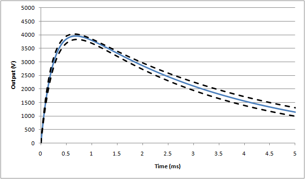
Trumpet curves

For general pumps, IEC1 requires the analysis to be performed at 2, 5, 11, 19 and 31 min (with similar points for ambulatory adjusted for the slower sample rate). That requires some 469 observation windows to be calculated, with 10 graph points.

The AAMI puts this on steroids: first it introduces a 10s sample interval, next it expands the range down to 1min, and finally requires the calculation to be made for all available observation windows. That results in some 47965 window calculations with 180 graph points

That said, the AAMI approach is not unreasonable: with software it is easy to do. It is possible to adopt a 10s sample interval from which a smooth trumpet curve is created (from 1 to 31 min as suggested). And, it is unclear why the IEC version uses only 2, 5, 11, 19 and 31min. It is possible that some pumps may have problem intervals hidden by the IEC approach.

So, somewhat unusually in this case, the recommended solution could be to adopt the AAMI version.

The balance (update 2019/09/20)

In figure 201.104b of IEC2, the balance in the diagram is shown as having four decimal places, while the note below says that a balance “accurate to” 5 decimal places “is required” for pumps with low minimum rates. This has a bunch of issues detailed below.

First, IEC/ISO Directive 2, Clause 28.5.4 “Notes to figures shall not contain requirements or any information considered indispensable for the use of the document”. So, again the writers have failed to follow the rules of writing standards.

Next, the note states that the balance should be “accurate to 5 decimal places”. It is most likely that the writers meant a resolution of 5 decimal places. To be accurate to 5 decimal places normally implies that the actual device displays an extra digit beyond, in other words it would require a balance that displays a resolution down to 0.000000g. Good luck finding that. Just to be pedantic (again) the note is missing any units. We assume it is grams based on the diagram, but …

Finally, ignoring the above issues and assuming the writers meant a resolution of 5 decimal places - research indicates that scales with a range of 220g and a resolution of 5 digits do exist, but they are extremely expensive and the specifications are not great. Noting that 0.00001g is effectively a resolution of 45 ppb (parts per billion) it looks like the balance manufacturers can achieve that resolution only with averaging, which could potentially affect the results. The scales would also be highly susceptible to vibration, and finally finding a calibration laboratory that is willing to check the device at that level of precision is likely to be very expensive if not impossible.

AAMI deleted this note. That says it all.

Back pressure

IEC1 and IEC2 require tests at the intermediate rate to be performed using a back pressure of ±100mmHg. This is easily done by shifting the height of the pump above or below the balance (approximately 1.5m = 100mmHg).

AAMI decided to change this to +300mmHg / -100mHg. The +300mmHg makes some sense in that real world back pressures can exceed 100mmHg. However, it makes the test overly complicated: it is likely to involve mechanical restriction which will vary with time and temperature and hence needs to be monitored and adjusted during tests up to 2hrs.

Recommended solution: The impact on accuracy is likely to be linearly related to pressure, so for example if there is a -0.5% change at +100mmHg, we can expect a -1.5% change at +300mmHg. The IEC test (±100mmHg) is a simple method and gives a good indication if the pump is influenced by back pressure, and allows direct comparison between different pumps. Users can estimate the error at different pressures using this value. Hence, the test at ±100mmHg as used in the IEC standards makes sense.

Update 2019/09/20: it has been pointed out that the above assumption of linearity between pressure and flow may not be valid. This suggests more work is required to investigate the effects and to develop a repeatable set up if higher pressures are required.

Pump types

In IEC1 and AAMI, there are 5 pump types in the definition of an infusion pump. The types (Type 1, Type 2 etc) are then used to determine the required tests.

In IEC2, the pump types have been relegated to a note, and only 4 types are shown. The original Type 4 (combination pumps) were deleted, and profile pumps, formally Type 5 are now referred to as Type 4. But in any case … it’s a note, and notes are not part of the normative standard.

Unfortunately this again seems to be a case of something half implemented. While the definition was updated the remainder of the standard continues to refer to these types as if they were defined terms, and even more confusingly, referring to Types 1 to Type 5 according to the definition in the previous standard. A newbie trying to read the standard would be confused by the use of Type 5 which is completely undefined, and by the fact that references to Type 4 pumps may not fit with the informal definition. A monumental stuff up.

In practice though the terms Type 1 to Type 5 were confusing and made the standard hard to read. It seems likely that the committee may have relegated it to a note with the intention of replacing the normative references with direct terms such as “continuous use”, “bolus”, “profile” and “combination” and so on. So for practical terms, users might just ignore the references to “Type” and hand write in the appropriate terms.

Drip rate controlled pumps

Drip rate controlled pumps were covered in IEC1, but appear to have been removed in IEC2. But … not completely - there are lingering references which are, well, confusing.

A possible scenario is that the authors were planning to force drip rate controlled pumps to display the rate in mL/hr by using a conversion factor (mL/drip), effectively making them volumetric pumps, and allowing the drip rate test to be deleted. The authors then forgot to delete a couple of references to “drop" (an alternative word to “drip”), but retained the test for tilting drip chambers.

Another possible explanation is that the authors were planning to outlaw drip rate controlled pumps altogether, and just forgot to delete all references. That seems unlikely as parts of the world still seem to use these pumps (Japan for example).

For this one there is no recommended solution - we really need to find out what the committee was thinking.

Statistical variability

Experience from testing syringe pumps indicates there is a huge amount of variability to the test results from one syringe to another, and from one brand to another, due to variations in “stiction”: the stop start motion of the plunger. And even for peristaltic type pumps the accuracy is likely to be influenced by the tube’s inner diameter, which is also expected to vary considerably in regular production. While this has little influence on the start up profile and trumpet curve shape, it will affect the overall long term accuracy.

Nevertheless, the standard only requires the results from a single “type test” to be put in the operation manual, leading to the question - what data should I put in? As it turns out, competitive pressures are such that manufacturers often use the “best of the best” data in the operation manuals, which is totally unrepresentative of the real world. Their argument is that - since everybody does it, … well … we have to do it. And, usually the variability is coming from the administration set or syringe, which the pump designers feel they are not responsible for.

In all three standards this issue is discussed (Appendix AA.4), but it is an odd discussion since it is disconnected with the normative requirements in the standard: it concludes that for example, a test on one sample is not enough, yet the normative parts only requires one sample.

Recommended solution (updated 2019/09/20)? Given that pumps, syringes and administration sets are placed on the market separately, it makes sense that separate standards (or separate sections in the standard) are developed for each part of the system. For example, tests could be developed to assess the variability of stiction in syringes with minimum requirements and declarations of performance if they are to be used with syringe pumps. Competitive pressure would then encourage manufacturers to work on making smoother action at the plunger.

Regulatory status

One might wonder why IEC 60601-2-24:2012 (EN 60601-2-24:2015) is yet to be adopted in Europe. In fact there are quite a few particular standards in the IEC 60601 series which have yet to be adopted in Europe. One possible reason is that the EU regulators are starting to having a close look at these standards and questioning whether they do, indeed, address the essential requirements. Arguably EN 60601-2-24:2015 does not, so perhaps there is a deliberate decision not to harmonise this and other particular standards that have similar problems.

The FDA , mysteriously, has no reference to either IEC and AAMI versions - mysteriously because it is a huge subject with lots of effort by the FDA to reduce infusion pump incidents, yet references to standards either formally or in passing seem to be non-existent.

Health Canada does list IEC 60601-2-24:2012, but interestingly there is a comment below the listing that “Additional accuracy testing results for flow rates below 1 ml/h may be required depending on the pump's intended use”, suggesting that they are aware of short comings with the standard.

Overall conclusion

Ultimately, it may be that the IEC committees are simply ill-equipped or structurally unsound to provide particular standards for medical use. The IEC is arguably set up well for electrical safety, with heavy representation by test laboratories and many, many users of the standards - meaning that gross errors are quickly weeded out. But for particular standards in the medical field, reliance seems to be largely placed on relatively few manufacturers, with national committees unable to provide plausible feedback and error checking. The result is standards like IEC 60602-2-24:2012 - full of errors and questionable decisions with respect to genuine public concerns. It seems we need a different structure - for example designated test agencies with good experience in the field, that are charged with reviewing and “pre-market” testing of the standard at the DIS and FDIS stages, with the objective of improving the quality of particular standards for medical electrical equipment.

Something needs to change!

ISO 14971: a madmans's criteria for acceptable risk

When auditing risk management files it can be a surprise to see a wide divergence in what companies deem to be acceptable risk. Some companies say a high severity event should be less than the proverbial one-in-a-million per year while others say one event in 100,000 uses is OK. Put on the same time scale, these limits have roughly a factor of around 1000 - something an industry outsider would scratch their head trying to understand.

Perhaps at the heart of this discrepancy is our inability to measure risk, which in turn means we can't test the decision making system to see if it makes any sense. Experienced designers know that anytime we create a “system” (software, hardware, mechanical), as much as 90% of initial ideas fail in practice. These failures get weeded out by actually trying the idea out - set up a prototype, apply some inputs, looks for the expected outputs, figure out what went wrong, feedback and try it all again until it works. We should be doing the same for the systems we use in risk management, but we can't: there are no reliable inputs. That allows many illogical concepts and outcomes to persist in everyday risk management.

But what if we ignore the problem on the measurement side, and tried to use maths and logic to establish a reasonable, broadly acceptable probability for, say, death? Would such an analysis lean towards the 1 in 100,000 per use or the more conservative 1 in 1,000,000 per year?  

It turns out that maybe neither figure is right - probably (pun intended)  the rate should be more like 1 in 100,000,000 events per year. Shocked? Sounds crazy? Impossible? Safety gone mad? Read on to find out how a madman thinks. 

Let’s start with the high end: “1 in 100,000 per use” - this looks reasonable from the point of view that 99.999% of patients will be fine. The raw probability of 0.001% is a tiny, tiny amount. And the patients are receiving significant benefit, so they should be prepared to wear a tiny bit of risk along the way. Every medical procedure involves some risk. 

Yes ... but ... no. It is seductive reasoning that falls apart with a bit of a bench test.

The first mistake is to consider the individual "risk" - that is, the individual sequence of events leading to harm - as a single case in isolation. From the patient's point of view that's irrelevant - what they perceive is the sum of all the risks in the device, together with all the risks from the many other devices that get used in the course of treatment. If every manufacturer used a limit of 1 in 100,000 per use for each hazardous situation associated with a high severity event, the cumulative risk would easily exceed what society would consider reasonable and even what is commercially viable. If the figure of 1 in 100,000 per use per sequence was accurate, a typical hospital would be dealing with equipment triggered high severity events on a daily basis.

Some might still feel that 0.001% is nevertheless an extremely small number and struggle to see why it's fundamentally wrong. To help grasp the cumulative concept it can be useful to consider an equivalent situation - tax. The amount of tax an individual pays is so tiny they might argue: what's the point in paying? And, to be honest it would not make any difference. It is a fraction of a fraction of a rounding error. Of course, we know that's wrong - a responsible person would not view their contribution but the cumulative result assuming everyone took the same action. It’s the same deal with a criteria of 0.001% per use: for an individual line item in a risk management file it is genuinely tiny and plausibly acceptable, but if every manufacturer used the same figure the cumulative result would be unacceptable.

The second mistake manufacturers (and just about everyone) does is to consider the benefit - as a tangible quantity - in the justification for acceptable risk. A manufacturer might say, OK yeah, there is a tiny bit of residual risk, but hey, look over here at all this wonderful benefit we are providing! Again a seductive argument, but fails to pass a plausibility test when thrown on the bench and given some light.

As detailed in a related article, benefit should not play any role in the criteria for acceptable risk: it’s a misdirection. Instead, our initial target should be to try and make all risks “negligible”. If, after this phase, significant risk remains and it is confirmed that further risk reduction is “not practicable”, we can turn to risk/benefit to justify releasing the device to market anyway. At this point the risk/benefit ratio might look important, but on close inspection the ratio turns out not to play any role in the decision: it’s just an end stage gate after all reasonable efforts in risk reduction have been applied. And in the real world, the benefit always far exceeds the risk, so the ratio itself is irrelevant.

So manufacturers often make two significant mistakes in determining acceptable risk (1) failure to appreciate cumulative risk, and (2) using benefit to justify higher rates.

Before we take our pitchforks out we need to keep in mind a mitigating factor - the tendency to overestimate probabilities. A common mistake is to record the probability of a key event in the sequence rather than the overall probability of harm. On top of this, safety experts often encourage manufacturers to overestimate probabilities, such as the failure rates for electronics. And when things get complicated, we opt for simplified models, such as assuming that all faults in a system lead to harm, even though this is clearly not the case. These practices often lead to probability estimates 10, 100 or even 1000 times higher than are actually observed in practice.

So the two mistakes often cancel each other out. But not always: every now and then a situation occurs where conflicts of interest (cost, competition, complexity, complacency … ) can push manufacturers genuinely into a higher probability zone which is unreasonable given that risk reduction is still feasible. The absence of good criteria then allows the decision to be deemed “acceptable”. So keep the pitchforks on hand just in case. 

In summary, the correct approach is first to try and make risks “negligible”, against criteria that takes into account the cumulative risk to the patient (operator, environment). If the residual risk is still significant, and further risk reduction is not practical, we can use the risk/benefit ratio to justify marketing the device anyway.

What, then, is "negligible" for death? Surely 1 in 1,000,000 per year is more than enough? Why would a mad-man suggest 1 in 100,000,000? 

Before delving into this question, there’s one more complication to address: direct and indirect harm. Historically, safety has been related to direct harm - from sources such as electric shock, mechanical movement, thermal, high energy, flow or radiation. This was even included in the definition of safety in the 1988 edition of IEC 60601-1 . One of the quiet changes in the 2005 edition was to adopt the broader definition of safety from ISO 14971 , which does not refer to direct or indirect, just “harm”. This change makes sense, as indirect harm such as failure to diagnose or treat are also valid concerns for society.

One problem though: acceptable risk for indirect harm is vastly more complex. This type of harm generally involves a large number of factors external to the medical device, including pre-existing illness, decisions by healthcare professionals, treatment parameters, other medical devices, drugs and patient action. The cumulative logic above is sound, but incredibly messy to extract a figure for, say, an appropriate failure rate for parts in a particular medical device that are associated with diagnosis and treatment.

This article is dealing a far simpler situation - say an infant incubator where the temperature control system goes crazy and kills the patient - and boils down to a simpler question: what is an acceptable probability of death for events which are 100% caused by the equipment?

It turns out that for high severity direct harm from electrical devices - electric shock, burn, fire, mechanical - the actual rates of death per device, per year, per situation are well below 1 in 100,000,000. Manufacturers (and regulators, standard writers, test agencies) are doing a pretty good job. And closer study of the events that do occur finds that few are due to random failure, but rather illegal imports that never met standards in the first place, or devices used far (far) beyond their designed lifetime, or use/modified far outside the intended purpose. In any case, evidence indicates that the 1 in 100,000,000 per year figure, while perhaps crazy, is absolutely achievable.

You can also turn the figures around and estimate the cumulative number of incidents if the proverbial one-in-a-million was the true rate. And it's not good news. For example, In the USA, there are 350 million people, assume 20 electrical devices per person, and each device has 10 high severity hazardous situations (for shock, fire, mechanical, thermal). That adds up to 70,000 deaths per year - just for electrical devices - far higher than society would consider reasonable if cost effective risk controls are available. Which obviously there are based on rates observed in practice.

So in general a target of 1 in 100,000,000 per year for death might not be such a crazy point of view after all.  

But to be honest, the precise targets are probably irrelevant - whether it is 1 in 1,000,000 or 100,000,000, the numbers are far too small to measure or control. It's great if we can get 1 in 100,000,000 in practice, but that seems to be more by luck than controlled design. 

Or is it?

One of the magical yet hidden aspects of statistics is how easily infinitesimally small probabilities can be created without much effort. All you need is a pack of cards or a handful of dice to demonstrate how this is done. Shuffle a deck of cards and you can be confident that no else in the history of mankind has or ever will ever order the pack in the same way. The number of combinations are just too big - a staggering 80,658,175,170,943,878,571,660,636,856,403,766,975,289,505,440,883,277,824,000,000,000,000 - yet there you are, holding it in your hand. 

In engineering it could be called the "sigma effect", the number of standard deviations we are away from the point of 50% failure. For a typical medium complexity device you need to be working around 5 sigma for individual parts to make the overall design commercially viable. Moving up a couple of notches to 7 sigma usually requires little in the way of resources, but failure rates drop to fantastically small values. By 8 sigma, Microsoft’s excel has heartburn even trying to calculate the failure rates, yet 8 sigma it is easily obtained and often used in practical design. If course, nobody actually measures the sigma directly - rather it is built into the margins of the design, using a 100mW resistor when the actual dissipation is 15mW, using a 5V±3% regulator for a microprocessor that needs 5V±10% . Good engineers roughly know where the “knee point” is (the point at which things start to cause trouble), and then use a good margin that puts it well into the 7+ sigma region.

In complex systems the large number of discrete parts can bring the system failure rate back into the realm of reality again, despite good design. Even so, negligible probabilities as appropriate to high severity events (e.g. death) can still be readily achieved by using redundant systems (independent protection) and other strategies.

Overall, engineers easily achieve these rates every day as evidenced by the low rates of serious events recorded in practice. .

But there is a catch: the biggest headache designers face is the whack a mole phenomena: try to fix problem A and problem B occurs. Fix B and C pops up. You could fix C but problem A partly sticks it's head up again. The designer then has to try and find a solution that minimises the various issues, trading off parameters in a spirit of compromise. In those situations, obtaining 7+ sigma can be impossible.

Non medical devices have both “whack a mole” problems and high risk issues, but it’s rare that they are related, So, designers usually have a clear separation of thinking: for the functional side compromise when needed, but for the high risk stuff don’t mess around, always go for the 7+ sigma solution.

In contrast, the “whack a mole” issues for medical devices are often related to the high risk functions, requiring compromise. As such it’s easy to get mixed up and assume that having been forced to accept a “low sigma” solution in one particular situation we can accept low sigma solutions elsewhere. In other words, compromise in one area easily bleeds into all decisions, ultimately leading to an organisational culture of justifying every decision on risk/benefit.

That’s the misdirection of risk/benefit raising it’s head again: the cart before the horse. We can justify low sigma based on risk/benefit only if there are no other feasible solutions around. And remember - feasible solutions are not always expensive - experience working with manufacturers of high risk devices frequently found that with a little push designers were able to create simple low cost solutions that achieve 7+ sigma without breaking the bank. The only thing holding them back was a false assumption that low sigma solution was acceptable in the first place.

For designers of high risk active medical devices, it takes good training and constant reminders to look for 7+ sigma solutions in the first instance, and only accept less when it’s “not practical” to do otherwise.

ECGs - 3 Lead tests

It is normal in ECG testing when confronted by large numbers of test permutations to simplify the approach on the assumption that one test is representative. For example, an input impedance test on V1 and V4 can reasonably be considered representative of tests on the other chest leads. And tests with the 10 lead cable is representative of tests with a 5 lead cable. 

One easy mistake though is to extend this to patient monitors that have the option to attach a 3 Lead cable.

In systems with 4, 5 or 10 electrodes, one of the electrodes is used as the "right leg drive", which is used for noise cancellation, both for mains and dc offsets. This function helps the system cope with dc offsets, mains noise (CMRR) and input impedance. 

In systems with 3 leads, there are two possible approaches: one is forget about noise cancellation and hope for the best. Another, more common is to use the displayed lead to decide which two leads are used for measurement, and have the other lead switch to the noise cancellation function. For example, if the normal default Lead II is shown on the display, electrode LA is not used (Lead II = LL - RA) , freeing up this lead for use as noise cancellation. 

You can check for the difference between these approaches by applying a dc offset (e.g. 300mV) to one of the electrodes, and then switching between Lead I, II and III and observing the baseline. If baseline remains constant, it is likely the manufacturer has used the "hope for the best" approach. If the baseline shows a transient when switching the lead displayed (e.g. Lead I to Lead II), it means the hardware circuit is switching the lead with the noise cancellation, and the high pass filter needs time to settle down. 

Either way, system with 3 lead options should be retested. The recommended test in IEC 60601-2-27 include: 

• sensitivity
• input impedance
• noise
• channel crosstalk
• CMRR
• pacemaker pulse (spot check)

For the remaining tests, it seems reasonable that tests on 10 lead configuration is representative. 

In reality though it is really up to the designer to know (and inform) about which tests can be considered representative. This is one of the weak points in IEC 60601 series in that there is no clear point of analysis for representative accessories and options, something which is discussed in another MEDTEQ article on accessories. 

MDD Essential Requirements

The following material is copied from the original MEDTEQ website, which was developed around 2009. It is noted that the proposed update to the European MDD addresses some of the points raised in this article. 

In Europe, manufacturers working under the Medical Device Directive (MDD) are given a legal "presumption of conformity" with essential requirements if they apply harmonized standards as published in the Official Journal. This feature is most often quoted as simply meaning that standards are voluntary; most people assume that essential requirements have the highest priority and must anyhow be fulfilled, in this context standards are just one way to show compliance.

Most people also assume the "presumption of conformity" only applies if the standard actually addresses the essential requirement; in other words, the presumption is not absolute. If standards don't cover an essential requirement or only provide a partial solution, the manufacturer is still obliged to provide additional solutions to ensure compliance with essential requirements.

While reasonable, this expectation is not actually supported by the directive. If the presumption was not absolute, we would need a mechanism, defined in the directive, to determine when the presumption is or is not effective. The expected mechanism would require each essential requirement to be analyzed and a formal decision made as to whether standards provide a complete solution, and if not, record the additional details necessary to provide that complete solution. The analysis would inevitably involve a characterization of the essential requirement for the individual device.

Consider for example, the application of essential requirement No. 10.1 (measurement functions) for a diagnostic ultrasound. To determine compliance we would need to compile the following information: 

• what measurement function(s) is/are there?
• for each measurement function, what is/are the intended purpose(s)?
• for each measurement function, what is an appropriate accuracy for the intended purpose(s)?
• for each measurement function, what is an appropriate test method for accuracy in design?
• for each measurement function, what is an appropriate test method for accuracy in production?
• for each measurement function, do the results of those test methods confirm the accuracy in design and production are suitable for the intended purpose(s)?

With this kind of detailed analysis, we can determine if standards genuinely provide a complete solution to the essential requirement, and also identify other solutions if the standards are incomplete. Given the huge range of medical devices, we know that standards struggle to provide a complete solution, and even those few that do address an essential requirement often provide only partial technical solutions which need to be supplemented with manufacturer specifications covering both design and production. Thus this analysis stage is expected to be extremely important for medical devices, and we can expect that the directive will specify exactly how to perform this analysis and what records must be maintained.

But when we look in the MDD to find what documentation must be kept (Annexes II ~ VII), we find surprisingly that there is no general requirement to document how essential requirements are fulfilled. Rather, each Annex says it is only if the manufacturer does not apply a harmonized standard that there is an obligation to document the solutions for essential requirements. This result is reinforced by Article 5, which says that member states must presume compliance with essential requirements if harmonized standards are applied. If these standards are inadequate, member states should take action to create standards, but there is no action required for the manufacturer.

Notified bodies have tried to fill this gap by insisting on an "essential requirements checklist". This checklist has now been formalized in the standard ISO/TR 16142. However, the checklist is really just a method of identifying which standards have been applied, and does not provide the analysis given above, nor record any formal decision as to whether a standard provides a complete "presumption of conformity", and if not, record the additional details necessary to provide a complete solution.  

The application of EN ISO 13485 and EN ISO 14971 were perhaps intended help to fill the gap; but there is a couple of legal problems: first is that neither of these standards, nor any management system standard actually meet the definition of a "harmonized standard" under the MDD. In principle, a harmonized standard is one that provides a complete technical solution (objective test criteria and test method), and should apply to the product, not the manufacturer (see Directive 98/34/EC, formerly 83/189/EEC).

More importantly, these standards have a key weak point: it is possible to argue under both ISO 13485 and ISO 14971 that analysis of essential requirements analysis should be performed, but there is no requirement for this analysis to be documented. Both standards limit the records to the results of the analysis, in particular ISO 14971 requires only the results of risk analysis to be recorded, not the technical analysis used to arrive at those results. While there are good reasons for this, it means that manufacturers can formally comply with these standards without ever actually documenting how essential requirements are met.

Independent observers would be somewhat bemused to find that there is no formal mechanism in the directive which forces manufacturers to document responses to important and difficult questions, such as:

• are low cost oscillometric based NIBPs suitable for home use with high blood pressure patients?
• are syringes with their highly variable stop/start action (stiction) suitable for use with infusion pumps when delivering critical drugs? 
• is the accuracy of fetal weight estimation by ultrasound suitable to make clinical decisions for cesarean procedures?
• can high powered hearing aids actually further damage hearing?

For each of the examples above, clinical literature exists showing they are real problems, yet it is rare to find these topics discussed in any detail in a manufacturer's technical file, quality system or risk management documentation, nor any formal conclusion as to whether the related essential requirement is met. The absence of such documentation is entirely in compliance with the law.

The reason for the apparent weakness in the directive can be found in the history behind the MDD. The original "new approach directives", first developed in the early 1980's were built on the assumption that published technical standards alone can reasonably assure compliance with the essential requirements, through the use of objective test methods and criteria (see 85/C 136/01 and 83/189/EEC). This is called the "general reference to standards" and requires that the standards provide " ... a guarantee of quality with regard to the essential requirements". The "general reference to standards" also says it should not be necessary to refer to "manufacturing specifications" in order to determine compliance, in other words, standards alone should provide the complete solution.

With this guarantee in place, an absolute presumption of conformity is reasonable. Manufacturers can be given a choice of either (a) applying the standard(s) and ignoring essential requirements, or (b) ignoring the standard(s) and applying essential requirements. You don't have to do both, i.e. apply standards and essential requirements. In general, essential requirements are intended to guide the standards writers, and only rarely need to be considered by those manufacturers that choose to ignore requirements in standards.  

For directives such as the LVD (low voltage), this worked well, as the standards could reasonably ensure compliance. But for other directives like the MDD, the range of devices and safety issues makes it impossible to develop comprehensive technical standards. As stated in 85/C 136/01:

"... in all areas in which the essential requirements in the public interest are such that a large number of manufacturing specifications have to be included if the public authorities are to keep intact their responsibility for protection of their citizens, the conditions for the "general reference to standards" approach are not fulfilled as this approach would have little sense"

Despite this problem, the EU went ahead and used the new approach framework for the MDD, as published in 1993. As the framework (Articles and Annexes) of CE marking directives was fixed based on Commission Decision EC COM(89) 209, the text related to the presumption of conformity and required documentation was adopted almost word for word. Thus, we can see in Annexes II ~ VII that manufacturers only need to refer to essential requirements if harmonized standards are not applied; in Article 5 the presumption of conformity is unconditional; and if there is doubt about standards assuring compliance then action is required by member states and not by manufacturers. While EC COM(89) 209 has now been updated twice (currently DECISION No 768/2008/EC), these parts of the MDD have not been yet updated to reflect the most recent framework.

So while competent authorities, notified bodies and even manufacturers might reasonably assume that the presumption of conformity is not absolute, the law doesn't support this. Moreover, the current informal approach, based on the essential requirement checklist, ISO/TR 16142, ISO 13485 and ISO 14971 also fails to effectively force manufacturers to look at each essential requirement in detail.

An interesting aside here is that the UK "transposition" of the MDD into national law includes a qualification that national standards provide a presumption of conformity with an essential requirement, "unless there are reasonable grounds for suspecting that it does not comply with that requirement". A slight problem, however, is that the UK is not allowed to do this: European law requires the local transposition to be effectively the same as the MDD, otherwise the whole concept of the common market and CE marking falls down. A secondary problem is that the UK law does not give any implementation details, such as who is authorized to decide, when such decision are required and what records are required. That the UK quietly added this modification to the MDD, despite being obviously illegal, clearly indicates the presumption of conformity is weak when applied to medical devices.   

So, is EU law at fault? Does it need to be amended to force manufacturers to analyze each essential requirement through a process of characterization, scientifically and objectively showing how the requirement is met, irrespective of standards?

Perhaps, but some caution is recommended. We need to keep in mind that CE marking may really just provide "clearance for sale", a function which needs to balance free flow of goods against risks, and which should wherever possible be based on legal certainty and objective technical specifications. Regardless of compliance with the directive, manufacturers are still liable for injury under the Product Liability Directive, which provides back up and incentive at least for serious and detectable issues. Competition also provides incentive in many other areas which are highly visible to the user, such as image quality in a diagnostic ultrasound.

Competition of course also has a darker side: pressure to reduce price and speed up market access. But, the reality is that manufacturers live in a competitive world. Like it or not, competition is a strong force and is a key reason why some of the difficult issues remain undocumented. Most manufacturers when questioned know well about these issues, but feel action is not required while the competition also takes no action. Even if we did force manufacturers to analyse essential requirements systematically, complex situations allow in bias, and the bias would tend towards keeping the status quo - it would take a lot of effort by notified bodies and regulators to detect and counter such bias working directly with each manufacturer.

In other words, forcing the analysis on manufacturers may not make much difference, and just add to compliance costs.

So, the answer here seems to be improving technical standards, forcing all manufacturers on to a "common playing field". In a round about way, Article 5 of the directive is perhaps on the best path: rather than expecting too much from manufacturers, member states should focus on creating standards that provide specific solutions (test methods and criteria) for individual medical devices.

For this to work, a critical point here is that standards committees need to take  Directive 98/34/EC seriously, creating standards that provide a complete, objective technical solutions for the product, rather than more management system standards without any specific technical details.

While we can never hope to address all safety issues in technical standards given the wide range of medical devices, it may be possible for member states to focus their efforts to those areas where product liability and competition are not effective at addressing known issues. In other words, it is not necessary for a standard to try and cover everything, just those areas which manufacturers are known to be weak.    

The main point is, the next time someone wants to discuss whether a standard provides a "presumption of conformity", make sure they have a cup of coffee ready, as the explanation will take a little time.

MDD - Retrospective application of harmonized standards: an investigation

Originally posted in October 2011. Due to the transfer, links to footnotes no longer operate. 

[PDF Version]

While significant discussion continues around the content of EN 60601-1:2006 (IEC 60601-1:2005), it is generally understood that in Europe as of June 1, 2012[1], the previous edition will be withdrawn, leaving only the new edition to provide the legal “presumption of conformity” against essential requirements.

Notified Bodies have indicated that this situation is in effect retrospective: all older designs that are still being sold will have to be re-verified against the new standard. This is based on the interpretation that the “presumption of conformity” only exists at a point in time when each individual device is placed on the market. Thus, in order for manufacturers to maintain compliance, they must continuously update the design taking into account current harmonized standards.

Although standards are voluntary, it is still expected that manufacturers evaluate compliance on a clause by clause basis. This ensures the manufacturer is aware of specific non-conformities, and can then choose to redesign or provide an appropriate justification as to why alternate solutions still meet the essential requirements. Thus the voluntary nature of harmonized standards has little impact on the amount of work associated with updates in standards, and in particular, work associated with retrospective application to existing designs.

Despite the apparent unity in Notified Bodies on this interpretation, the MDD does contain text that calls this interpretation into question. Moreover, the implications of broad retrospective application may not have been fully considered by Notified Bodies.

The preliminary "whereas" section of the Medical Device Directive (MDD) includes the following paragraph:

“Whereas the essential requirements and other requirements set out in the Annexes to this Directive, including any reference to ‘minimizing’ or ‘reducing’ risk must be interpreted and applied in such a way as to take account of technology and practice existing at the time of design and of technical and economical considerations compatible with a high level of protection of health and safety;”

Later, in a paragraph associated with harmonized standards, this is repeated again:

"… essential requirements should be applied with discretion to take account of the technological level existing at the time of design and of technical and economic considerations compatible with a high level of protection of health and safety"

These statements appear to indicate that the presumption of conformity may exist at the time of design, rather than the time of placing on the market. If so, this would remove the retrospective nature of standards, and conflict with the advice of Notified Bodies. While the “high level of protection” part is open to interpretation, it appears that the intention was to say that essential requirements, standards and risk should be considered to apply at the time of design, unless there are some serious concerns. For example, if incidents in the market led to changes in standards or state of the art, such changes could be considered reasonable even for old designs.

Unfortunately, this “time of design” statement lacks further legal support. In the core part of the directive (articles, annexes) the phrase is not repeated. It also appears that the “whereas” section has not been transposed into national law (UK law, for example, does not use the phrase). The forward of EN ISO 14971 does repeat the above statement that "risk" must be assessed “at the time of design”, and this is also clarified in again in Annex D.4 in the same standard. But since these references are hidden away from the normative text, again they are often overlooked. So if the authors of the MDD really did intend the presumption of conformity to apply at the "time of design", there is considerable room for the EU to improve on implementation to provide greater legal certainty.

So, we are left with the task of finding out if retrospective application is feasible. An investigation finds that there are three key areas: the first looks at the unusually large number of standards that apply to medical devices; the second considers the case of “brand new” standards (without any transition period), and the third is the impact of requirements that apply to the manufacturer, as opposed to the device.  

Notified bodies have tended to highlight the retrospective aspect on high profile product standards undergoing transition, such as EN 60601-1:2006. But they have been very weak in enforcing the retrospective rule for all harmonized standards.

This is not a reflection of poor quality work by Notified Bodies, but rather the sheer impracticality of the task. While other directives may have more standards, the MDD is perhaps unique in the large number of standards that can apply to a single "product". Under the Low Voltage Directive, for example, two to three standards would typically apply to an electrical appliance such as a toaster or washing machine, keeping retrospective application in the realm of feasibility. Other high profile directives don't use the phrase “at the time of design” .

In contrast, a typical medical electrical device will have at least 10 harmonized standards, and Appendix 1 of this document lists some 26 harmonized standards that would apply to a typical full featured patient monitor.

Keeping on top of all these standards retrospectively is arguably beyond what can reasonably be expected of manufacturers. Benefits from new standards would be offset by adverse effects such as impeding innovation and increasing costs of medical devices. Another less obvious effect is that it tends to make standards less effective: recognizing the heavy burden, third parties often allow simplifications to make the standards easier to apply retrospectively, but these simplifications set up precedents that can take many years to reverse. 

Not only are there a large number of standards being regularly updated, there are also many “brand new” standards which are harmonized without any transition period. This poses a special case where retrospective application is impossible, since a manufacturer cannot know when a standard will be harmonized. In a sense, the standard becomes instantaneously effective on the day it is first published in the Official Journal.

In literature associated with EN 60601-1:2006 (IEC 60601-1:2005), it has been pointed out that the original standard has been around for many years, thus manufacturers have no excuse for further delays beyond June 2012. But this is again an example where only high profile standards are being considered, not the full range of both harmonized and non-harmonized standards.

The “no excuse” interpretation implies that manufacturers must watch IEC or ISO publications, anticipate and prepare for harmonization. But this is not only unfair since there are many IEC and ISO standards that never get harmonized, it is also logistically impossible. There are many examples where the time from first publication as IEC or ISO to publication in the Official Journal is less than 18 months[2]; no reasonable law could expect implementation in such a short time, particularly in the context of retrospective application. Moreover, the simple logistics of CE marking (such as the declaration of conformity, technical file) would be impossible arrange in a single day when the standard first appears in the Official Journal.

The case of “brand new” standards alone provides simple, unarguable evidence that the presumption of conformity cannot apply at the time of placing on the market, without violating the principles of proportionality and legal certainty[3].

A more complex situation exists with manufacturer requirements, usually in the form of management systems. EN 60601-1:2006 highlights these problems as it has both product and manufacturer requirements in the same standard. Manufacturer requirements are those which require the manufacturer to take some specific action indirect to the product; while these actions are intended to have an influence on the product they are often several layers removed, such as the retention of qualification records of persons involved in the design.   

Historically, the new approach directives were based on product requirements, and it is arguable that areas of the directive have not been fortified to handle manufacturer requirements. Even the definition of a harmonized standard is “a specification contained in a document which lays down the characteristics required of a product …”[4], and thus appears not to have provision for manufacturer requirements.

Since the principles of free movement, essential requirements the presumption of conformity all  apply to the device, it is obvious management systems alone cannot be used to provide a presumption of conformity; rather it is the design specifications, verification records and other product related documents output from the management system which provide the main evidence of conformity.

If a harmonized management system standard is updated, the question then arises about the validity of product related documents which were output from the old system. In other words, whether the older documents still provide a presumption of conformity. Moreover, if a “brand new” management system standard is harmonized (such as EN 62304), the question arises whether manufacturers are required to apply the management system in retrospect for older designs.

This is very different to product requirements. A change in product requirements might be annoying, but generally limited in the amount of resources required for re-testing or redesign for specific technical issues. In contrast, a change in a management system can invalidate large amounts documentation and  trigger a massive amount of rework, far beyond what is reasonable to achieve the objective of health and safety. Manfacturer requirements are clearly written to apply at the time of design: the costs are relatively small if applied at the time of design, whereas as the implementation after the design is complete can be incredibly high.

Consider for example, a manufacturer that has an older programmable system, but did not record whether the persons validating the design were not involved in the design, as required by EN 60601-1:2006, Clause 14.11. A strict, retrospective interpretation would find all the validation tests invalid, and force the manufacturer to repeat them all again at great cost.

Thus, while less straightforward, management systems also provide a fairly strong argument that the presumption of conformity applies at the time of design.

In practice, most Notified Bodies take a flexible view on retrospective application of management systems, using common sense, taking into account the amount of work required, and focusing on high level documents associated with high profile standards.

Also with respect to “brand new” standards, Notified Bodies often apply an informal transition period of 3 years from the time a standard first harmonized, recognizing that immediate application is impractical.

While these relaxations are reasonable, they are not supported by the law. This is not a case where vagueness in the law requires Notified Body interpretation to fill in the details; this is in a sense a simple question of when the presumption of conformity applies. The answer, whatever it is, must be universally applied. It is not possible to apply one interpretation to EN 60601-1 and another to EN 62304. All harmonized standards must be treated equally.

With the current law, the only practical universal interpretation is that the presumption of conformity applies at the time of design, as indicated by the “whereas” section of the MDD.

It is worth to note that no official document endorsed by the EU commission indicates that retrospective application is required. This is unlikely to happen as documents issued by the EU are usually carefully vetted by the lawyers, a process which is likely to raise similar concerns as discussed above. In particular, the situation with “brand new” standards (standards without a transition period) will make the commission wary of formally declaring standards to be retrospective.

Also, it is a well established regulatory requirement (e.g. clinical data, EN ISO 13485, EN ISO 14971) that post market monitoring includes the review of new and revised standards.  Thus, the “time of design” interpretation does not imply manufacturers can completely ignore new standards. But importantly, the flexibility in decisions to apply new standards to older designs is made by the manufacturer, not the Notified Body.   

The “time of design” interpretation is not without problems. Designs may take many years to finalize, so the term “time of design” obviously requires clarification. It could also lead to products falling far behind state the art, or failing to implement critical new requirements quickly. Even using the “time of design” interpretation, “brand new” standards still pose a challenge to manufacturers, since it can be impractical to apply even to current designs. So, more work is required.  

But in the context of EN 60601-1:2006, a “time of design” interpretation would act as a pressure relief valve not only for manufacturers, but for all parties involved who are struggling to apply such a large new standard retrospectively.

Appendix 1: Harmonized standards applicable to a patient monitor

The following is a list of harmonized standards which are currently applicable to a typical full featured patient monitor including accessories. Items shown in brackets are standards which are expected to replace the existing standard or are already in transition.

EN 980

EN 1041

EN 1060-1

EN 1060-3

EN 1060-4 (ISO 81060-2)

EN ISO 9919 (EN 80601-2-61)

EN ISO 10993-1

EN ISO 12470-1

EN ISO 12470-4 (EN 80601-2-56)

EN ISO 13485

EN ISO 14971

EN ISO 17664

EN ISO 21647

EN ISO 20594-1

EN 60601-1

EN 60601-1-2

EN 60601-1-4 (EN 60601-1/Clause 14)

EN 60601-1-6

EN 60601-1-8

EN 60601-2-27

EN 60601-2-30 (EN 80601-2-30)

EN 60601-2-34

EN 60601-2-49

EN 60601-2-51

EN 62366

EN 62304
 

[1] The actual date will depend on particular standards

[2] See EN 62366 (Usability Engineering) which has only 13 months from publication as IEC to listing in the Official Journal.

[3] As required by the “Treaty of the European Union” 

[4] See directive 98/34/EC

IEC 60601-2-25 Clause 201.12.4.103 Input Impedance

The input impedance test is fairly simple in concept but can be a challenge in practice. This article explains the concept, briefly reviews the test, gives typical results for ECGs and discusses some testing issues. 

What is input impedance? 

Measurement of voltage generally requires loading of the circuit in some way. This loading is caused by the input impedance of the meter or amplifier making the measurement. 

Modern multimeters typically use 10MΩ input for dc measurements and 1MΩ for ac measurements. This high impedance is usually has negligible effect, but if the input impedance is similar to the circuit impedance significant errors can result. For example, in the circuit shown, the real voltage at Va should be exactly 1.000Vdc, but a meter with 10MΩ input impedance will cause the voltage to fall by about 1.2%, due to the circuit resistance of 240kΩ.   

Input impedance can be derived (measured) from the indicated voltage if the circuit is known and resistances are high enough to to make a significant difference relative to noise and resolution of the measurement system. For example in Figure 1, if the supply voltage, Rs and Ra are known, it is possible to work back from the displayed value (0.9881) and calculate an input impedance of 10MΩ. 

The test

The test for ECGs is now largely harmonised in all the IEC and ANSI/AAMI standards, and uses a test impedance of 620kΩ in parallel with 4.7nF. Although the requirement is written with a limit of 2.5MΩ minimum input impedance, the actual test only requires the test engineer to confirm if the voltage has dropped by 20% or less, relative a the value shown without the test impedance.  

ECGs are ac based measurements so the test is usually performed with an sine wave input signal. Input impedance can also change with frequency, so the IEC standards perform the test at two points: 0.67Hz and 40Hz. Input impedance test is also performed with ±300mV offset, and repeated for each lead electrode. That makes a total of 2 frequencies x 4 conditions (reference value + open + 2 offsets) x 9 electrodes = 72 test conditions for a 12 Lead ECG.  

Typical results

Most ECGs have the following typical results:   

• no measurable reduction at 0.67Hz
• mild to significant reduction at 40Hz, sometimes close to the 20% limit
• not affected by ±300mV dc offset 

Issues, experience with the test set up and measurement

Although up to 72 measurements can be required (for a 12 Lead ECG), in practice it is reasonable to reduce the number of tests on the basis that selected tests are representative. For example, Lead I, Lead III, V1 could be comprehensively tested, while Lead II, V1 and V5 could be covered by spot checks at 40Hz only, without ±300mV.

In patient monitors with optional 3, 5, and 10 lead cables, it is normal to test the 10 lead cable as representative. However, for the 3 lead cable there can be differences in the hardware design that require it to be separately tested (see this MEDTEQ article on 3-Leads for more details).  

The test is heavily affected by noise. This is a result of the CMRR being degraded due to the high series impedance, or more specifically, the high imbalance in impedance. As this CMRR application note shows, CMRR is heavily dependent on the imbalance impedance. 

An imbalance of 620kΩ is 12 times larger than the CMRR test, so there is proportional degrading of the CMRR by the same factor of 12. This means for example that with a typical set up having 0.1mm (10µV@10mm/mV) mains noise for typical tests, would increase to 1.2mm of noise once the 620kΩ/4.7nF is in circuit. 

For the 0.67Hz test, the noise appears as a think line. It is possible consider the noise as an artefact and measure the middle point this think line (that is, ignore the noise). This is a valid approach especially as at 0.67Hz, there is usually no measurable reduction, so even increased measurement error from the noise, it is a clear "Pass" result. 

However, for the 40Hz test there is no line as such, and the noise is similar frequency resulting in beating, obscuring the result. And the result is often close to the limit. As such, the following is steps are recommended to minimise the noise:  

• take extra care with the test environment, check grounding connections between the test circuit, the ECG under test, and the ground plate under the test set up
• During measurement, touch the ground plate (this has often been very effective)
• If noise still appears, use a ground plate above the test set up as well (experience indicates this works well)
• Enable the mains frequency filter; this is best done after at least some effort is made to reduce the noise to using one or more of the methods above to avoid excessive reliance on the filter
• Increase to a higher printing speed, e.g. 50mm/s 

Note that if the filter is used it should be on for the whole test. Since 40Hz is close to 50Hz, many simple filters have a measurable reduction at 40Hz. Since the test is proportional (relative), having the filter on does not affect the result as long as it is enabled for both the reference and actual measurement (i.e. with and without the test impedance). 

ECG Leads - an explanation

From a test engineer's point of view, it is easy to get confused with LEADS and LEAD ELECTRODES, because for a typical electrical engineer, "lead" and "electrode" are  basically the same thing. But there is more confusion here than just terminology. How do they get a "12 lead ECG" for a cable with only 10 leads? Why is it that many tests in IEC standards ask you to start with RA, yet the indication on the screen is upside down? Why is it that when you put a voltage on RA, a 1/3 indication appears on the V electrodes?

Starting with this matrix diagram, the following explanation tries to clear up the picture:

LEAD ELECTRODES are defined as the parts that you can make electrical connection to, such as RA, LA, LL, V1 and so on. On the other hand, LEADS are what the doctor views on the screen or print out.

There are a couple of reasons why these are different. Whenever you measure a voltage it is actually a measurement between two points. In a normal circuit there is a common ground, so we often ignore or assume this second reference point, but it's always there. Try and measure a voltage using one point of connection, and you won't get far.

ECGs don't have a common reference point, instead physicians like to see different "views" of the heart's electrical activity, each with it's own pair of reference points or functions of multiple points. One possibility would be to always identify the points of reference, but this would be cumbersome. Instead, ECGs use labels such as "Lead I" or "Lead II" to represent the functions.

For example "Lead I" means the voltage between LA and RA, or mathematically LA - RA. Thus, a test engineer that puts a positive 1mV pulse on RA relative to LA can expect to see an inverted (negative) pulse on Lead I.

Leads II and III are similarly LL-RA and LL-LA. 

The waveforms aVR, aVL and aVF are in effect the voltages at RA, LA and LL respectively, using the average of the other two as the second reference point.

Waveforms V1 ~ V6 (where provided) are the waveforms at chest electrodes V1 ~ V6 with the average of RA, LA and LL as the second reference point.

These 12 waveforms (Lead I, II, III, aVR, aVL, aVF, V1 ~ V6) form the basis of a "12 lead ECG".

Whether you are working with IEC 60601-2-27 or IEC 60601-2-51, you can refer to the diagram above or Table 110 in IEC 60601-2-51 which shows the relationship between LEAD ELECTRODES and LEADS.

Finally, you may ask what is RL (N) used for? The typical mistake is to assume that RL is a reference point or ground in the circuit, but this is not correct. In most systems, RL is not used for measurement. Rather it is used for noise cancellation, much like noise cancelling headphones, and is often call a "right leg drive". It senses the noise (usually mains hum) on RA/LA/LL, inverts and feeds back to RL. For testing IEC 60601-1, engineers should take note of the impedance in the right leg drive, as this tends to be the main factor which limits dc patient currents in single fault condition.

Exercise (test your understanding)

To check your understanding of the matrix, try the following exercise: if a 1mV, positive pulse (e.g. 100ms long) was fed to RA with all other inputs grounded, what would you expect to see on the screen for each lead? The answer is at the end of this page.

Other related information (of interest)

In years gone by, the relationship (matrix) above was implemented in analogue circuits, adding and subtracting the various input voltages. This meant that errors could be significant. Over time, the digital circuits have moved closer and closer to the inputs, and as well the accuracy of remaining analogue electronics has improved, which means it is rare to get any significant error in modern equipment. The newest and best equipment has a wide range high resolution input analogue to digital conversion very close to the input, allowing all processing (filtering as well as lead calculation) to be performed in software.

It is interesting to note that mathematically, even though there are 12 Leads, there are only 8 "raw" waveforms. Four of the 12 waveforms can be derived from the other 8, meaning they are just different ways of looking at the same information. For example, Lead III = Lead II - Lead I. It makes sense, since there are only nine points electrical connections used for measurement (remember, RL is not used for measurement), and the number of raw waveforms is one less than the number of measurement points (i.e. one waveform requires 2 measurement points, 2 waveforms requires at least 3 points, an so on). This is the reason why systems can use 8 channel ADC converters, and also why the waveform data used IEC 60601-2-51 tests (such as CAL and ANE waveforms) uses just 8 channels of raw data to create a full 12 Lead ECG.

Although the standard usually indicates that RA is the first lead electrode to be tested, if you want to get a normal looking waveform from a single channel source, it is best to put the output to LL (F) so that you get a positive indication on Lead II. Most systems default to a Lead II display, and often use Lead II to detect the heart rate. If your test system can select to put the output to more than one lead electrode, select LA and LL, which will give a positive indication on Lead I and Lead II (although Lead III will be zero).

Results of the exercise (answer)

If a +1mV pulse was applied to RA only, the following indications are expected on the screen (or printout). If you did not get these results or do not understand why these values occurred, go back and study the matrix relationships above. For the Lead electrodes, use RA = 1 and for all other use 0, and see what the result is.

Lead	Indication direction	Indication amplitude
I	Negative	1.00mV
II	Negative	1.00mV
III	None	None
aVR	Positive	1.00mV
aVL	Negative	0.50mV
aVF	Negative	0.50mV
V1 ~ V6	Negative	0.33mV

Defibrillator Proof Testing

(this material is copied across from the original MEDTEQ website, developed around 2009)

Introduction

Defibrillator proof testing is common for equipment associated with patient monitoring, HF surgical (neutral electrode) and ECG, and any device that may remain attached to a patient during defibrillation. In order to speed up delivery of the defibrillator pulse, it is desirable to leave many of the applied parts connected to the patient; thus such applied parts should be able to withstand a pulse without causing an unacceptable risk. In general, a defibrillator proof specification is optional, however, particular standards may specify that it is mandatory (for example, ECG related).

This section covers the following topics related to defibrillator proof testing (defib testing):

Potential hazards / Defibrillator pulse characteristics / Design considerations / Practical testing / Test equipment calibration

Potential hazards

The potential hazards associated with the use of a defibrillator when other equipment is connected to the patient are:

• permanent damage of medical equipment attached to the patient
• loss of critical data, settings, operation for monitoring equipment attached to the patient
• inability of monitoring equipment to operate to determine the status of the patient (after defibrillation)
• shunting (loss) of defibrillator energy
• conduction of defibrillator energy to the operator or unintended locations in the patient

All of these are addressed by IEC 60601-1:2005 (Clause 8.5.5), although particular standards such as IEC 60601-2-27 (ECG, monitoring) may specify more detail in the compliance criteria. The tests identify two paths in which the defibrillator pulse can stress the equipment: 

• Common mode: in this case the voltage typically appears accross patient isolation barriers associated with Type F insulation.
• Differential mode: in this case the voltage will appear between applied parts

Design and testing considerations for both of these modes are detailed below.

Defibrillator pulse characteristics

For the purpose of testing other than the shunting of energy, the standard specifies a defib pulse sourced from a 32uF capacitor, charged to 5000V (equivalent to 400J), which is then discharged via series inductor (500µH, max 10Ω). For copyright reasons, please refer to the standard for the actual circuit diagram.

These values are historically based on older style "monophasic" defibrillators that were designed to deliver a maximum of 360J to the patient with peak voltages around 5kV and peak current of 50A. Assuming the inductor has a resistance of 5Ω, and the remaining components are nominal values, the simulated nominal waveform is as follows (this simulation is based on differential step analysis, a excel sheet using the simulation allowing component variation can be downloaded here): 

 

The drop in peak voltage from the expected 5000V is due to the series resistance in the inductor creating a divider with the main 100Ω resistor. In this case, since 5Ω was assumed there is ~5% drop. The rise time of this waveform is mainly influenced by the inductor/resistor time constant (= L/R = 500µH / 105Ω = ~ 5µs), while the decay time is largely influenced by the capacitance/resistance time constant  (32µF/105Ω = ~ 3.2ms). Again using ideal values (and 5Ω for inductor resistance), the expected values are:

Peak voltage, Vp = 4724V
Rise time (time from 30% -> 90% of peak), t_r = 9.0µs
Fall time (start of waveform to to 50% of peak), t_f = 2.36ms

The leading edge of the ideal waveform is shown in more detail here:

Modern defibrillators use "biphasic" waveforms with much lower peak voltages, and lower energy may be considered safer and more effective (see this article for an example). Also, as the standard points out, in the real world the voltage that appears in applied parts will be less than that delivered by the defibrillator. However, the standard continues to use the full high voltage monophasic pulse (tested at both polarities) for the basis of the test. In practice this often has little effect since the Type F insulation in equipment is usually designed to withstand 1.5kVrms for 1 minute, which is much more tough than 5kV pulse lasting for a few milliseconds. However, occasional problems have been noted due to spark gaps positioned across patient insulation areas with operating voltages around 3kV. When tested in mains operation, there is no detectable problem, but when tested in battery operation breakdown of the spark gap can lead to excess energy passing to the operator (see more details below). 

For the energy reduction test (IEC 60601-1,  8.5.5.2) the standard specifies a modified set up using a 25mH inductor, rather than the 500µH specified above. Also, the inductor resistance is fixed at 11Ω. This leads to a much slower rise time in the waveform, and also a significant reduction in the peak voltage:

For this test, the nominal waveform parameters are:

Peak voltage, Vp = 3934V
Rise time (time from 30% -> 90% of peak), t_r = 176µs
Fall time (start of waveform to to 50% of peak), t_f = 3.23ms

As discussed in the calibration section below, it can be difficult to realise these waveforms in practice due to difference between component parameters measured at low current, voltage and frequency (e.g. an LCR meter), compared to actual results at high current, voltage, and frequency.

Design considerations

The following considerations should be taken by designers of equipment for defibrillator protection, and also verification test engineers (in-house or third party laboratories), prior to performing the tests to ensure that test results are as expected.

A) Common mode insulation

Solid insulation (wiring, transformers, opto-couplers)

During the common mode test, the Type F patient isolation barrier will most likely be stressed with the defib pulse. However, although the peak defib voltage is higher than F-type applied part requirements, for solid insulation an applied voltage of 1.5kVrms applied for 1 minute (2.1kVpeak) is far more stressful than 5kV pulse where the voltage exceed 2kV for less than 3ms. Thus, no special design consideration is needed.

Spacing (creepage, clearance)

According to IEC 60601-1, it is necessary to widen the applicable air clearance from 2.5mm to 4.0mm for applied parts with a defibrillator proof rating, which matches the limit for creepage distance. Since in most cases the minimum measured creepage and clearance are at the same point (e.g. between traces on a PCB), this often has little effect. However, in rare cases, such as in an assembled device, clearances may be less than creepage distances.

EMC bridging components (capacitors, resistors, sparkgaps)

For EMC, it is common to have capacitors, resistors and sparkgaps bridging the patient isolation barrier. In general, there are no special concerns since the insulation properties (1.5kVrms, 1min) ensure compliance with 5kVp defib pulse, and impedance of these components is also far higher than needed to ensure compliance with leakage current limits. Based on simulations, a 10nF capacitor or a 150kΩ resistor would result in a borderline pass/fail result for the test for operator shock (1V at the Y1-Y2 terminals), but such components would result in a leakage current in the order of 1mA during the mains on applied part test, a clear failure.

The one exception is the spark gap: provided the rating is above 5kV, there is no concern, however, cases have been noted of spark gaps rated at around 3kV, and breaking down during the test. This is of particular concern for patient monitors utilising battery operation, since in this battery operation the energy can be transferred to the operator via the enclosure (in mains operation, the energy flows to earth and causes no harm).

Although there are arguments that the 5kV peak is too high, unfortunately this is still specified in the standard, and it is recommended that any spark gaps bridging the patient isolation barrier have a rated voltage which ensures no breakdown at 5kV. In order to allow for tolerance, this may mean using a spark gap rated at around 6kV.

B) Differential insulation (general)

For equipment with multiple applied parts (such as a patient monitor), differential insulation is needed to ensure compliance with the differential test (exception is the ECG function, which is discussed below) and the energy reduction test. While this insulation can be provided in the equipment, typical implementation relies on insulation in the sensor itself, to avoid the need to design multiple isolated circuits. Typically, common temperature sensors, IBP transducers and re-useable SpO2 probes provide adequate insulation, given the relatively light electrical stress of a defib pulse (again, although it is high peak voltage, the short duration means most modern material have little problem withstanding a pulse).

However, it can be difficult for a manufacturer of a patient monitor to provide evidence of conformity for all the sensors that might be used with a monitor, since a large range of sensors can be used (in the order of 20-100), as optional accessories, and these are manufacturered by other companies. In some cases, the manufacturer of the patient monitor does not actually specify which sensors can be used, simply designing the equipment to interface with a wide range of sensors (e.g. temp, IBP, ECG electrodes).  

Currently, IEC standards for patient monitors treat the device and accessories as one complete item of "equipment" . This does not reflect the actual market nor the current regulatory environment, which allows the separation of a main unit and sensors, in a way which allows interchangeability without compromising safety. Although a manufacturer of a patient monitor may go to the extreme of testing the monitor with all combinations of sensors, this test is relatively meaningless in the regulatory environment since the patient monitor has no control over design and production of the sensors (thus, for example, a sensor manufacturer may change the design of a sensor without informing the patient monitor, invalidating the test results).

In the modern regulatory environment, a system such as this should have suitable interface specifications which ensures that the complete system is safe and effective regardless of the combination of devices. To address the defibrillation issue, for example, sensor manufacturers should include a specification to withstand a 5kV defib pulse without breakdown between the applied part of the sensor (e.g. probe in in saline) and the internal electrical circuit. It is expected that manufacturers of sensors are aware of this issue and are apply suitable design and production tests. IEC standards should be re-designed to support this approach.

To date there are no reported problems, and experience with testing a range of sensors has found no evidence of breakdown. Due to failure of the standards to address this issue appropriately, test laboratories are recommended to test patient monitor equipment with the samples selected by the patient manufacturer, rather than the complete list of accessories.

There is a question about disposable SpO2 sensors, since the insulation in the sensor is not as "solid" as non-disposable types. However, provided all other applied parts have insulation, this is not a concern.

C) Differential protection (ECG)

The ECG function differs in that direct electrical connection to the patient is part of normal use. Thus, it is not possible to rely on insulation for the differential test, and there are several additional complications.

Manufacturers normally comply with the basic differential requirement by using a shunt arrangement: a component such as gas tube spark gap or MOV is placed in parallel with the leads, and shunts the energy away from the internal circuits. Since the clamping voltage of these devices is still relatively high (50-100V), series resistors after the clamping device are still needed to prevent damage to the electrical circuit. These resistors combine with input clamping diodes (positioned at the input of the op-amp) so that the remaining current is shunted through the power supply rails.

Early designs placed the clamping devices directly across the leads, which led to the problem of excessive energy being lost into the ECG, a hazard since it reduces the effectiveness of the defib pulse itself. This in turn led to the "energy reduction test", first found in IEC 60601-2-49 (only applicable to patient monitors), then part of IEC 60601-2-27:2005 and now finally in the general standard (applicable to all devices with a defib rating). To comply with this requirement, the ECG input needs additional current limiting resistors before the clamping device, so a typical design will now have resistors before and after the clamping device. From experience, resistor values of 1kΩ will provide a borderline pass/fail result, higher values of at least 10kΩ are recommended (50kΩ seems to be a typical value). While patient monitors under IEC 60601-2-49 have dealt with this requirement for many years, diagnostic ECGs will also have to comply with this requirement after the 3rd edition becomes effective. This may result in conflicts since many diagnostics ECGs try to reduce the series impedance to improve signal to noise ratios (e.g. CMRR), and may not have any resistors positioned ahead of the clamping device.

The protection network (resistors, shunt device) can be placed in the ECG lead or internal to the equipment. The circuit up to the protection network should be designed with sufficient spacing/insulation to withstand the defibrillator pulse. The resistors prior to the shunt device should be of sufficient power rating to withstand multiple pulses, taking into account normal charging time (e.g. 30s break) in between pulses.

Figure: typical ECG input circuit design for defibrillator protection

An additional problem with ECG inputs is due to the low frequency, high pass filter with a pole situated around 0.67Hz for "monitoring" filter setting, and 0.05Hz for the "diagnostic" setting. A defibrillator pulse will saturate this filter (base line saturation), preventing normal monitoring for extended periods., This is a serious hazard if the ECG function is being used to determine if the defib pulse was successful. Manufacturers typically include a base-line reset function in either hardware and/or software to counter this problem. There have been cases where in a "diagnostic" setting, the baseline reset is not effective (due to the large overload), and some manufacturers have argued that the "diagnostic" mode is a special setting and therefore the requirements do not apply. However, this argument is weak if analyzed carefully using risk management principles. Even if the probability of defibrillating the patient when the equipment is in the "diagnostic setting" is low (e.g. 0.01), the high severity (death) would make it unacceptable not to provide a technical solution.

Finally, there is a testing in the ECG particulars (IEC 60601-2-25, IEC 60601-2-27) which involves use of real gel type ECG electrodes. This test is intended to determine the effects of current through the electrodes. Excessive current can damage the electrodes, causing an unstable dc offset that prevents monitoring and hence determination of a sucessful defibrillation - a critical issue. While it has all good intentions, this test unfortunately is not well designed, since it is not highly repeatable and greatly dependent on the electrodes tested. In the real world, ECG equipment is used with a wide variety of electrodes which are selected by the user, and not controlled by the manufacturer. There is little logical justification for testing the ECG with only one type of electrode. Fortunately, the energy reduction test has largely made this a irrelevant issue - in order to comply with that test, equipment now typically includes series resistors of at least 10kΩ. This series resistance also reduces the current through the gel electrodes. Experience from tests indicates that equipment with series resistors of 10kΩ or higher, there is no detectable difference between the test with electrodes and without electrodes, regardless of the type of electrode. Logically, standards should look at replacing this test with a measurement of the current, with a view to limit this to a value that is known to be compatible with standards for get electrodes (e.g. ANSI/AAMI EC12:2000 Disposable ECG electrodes, 3ed.).  

Practical testing

Simplification

Testing of a single function device is relatively simple. However, testing of a multiparameter patient monitor can explode the potential number of tests. In order to reduce the number of individual tests, it is possible to use some justification based on typical isolation structures and design:

• common mode test: this test can be performed with all applied part functions shorted together, similarly with all accessible parts (including isolated signal circuits) shorted together. If applied parts such as temp/SpO2/IBP all connect into a single circuit, make your applied part connection directly to this circuit rather than wasting time with probes in saline solution. Ensure that the test without mains connection is performed if battery powered, this will be the worst case. If with this simplification, the Y1-Y2 result is <1V, then logically tests to individual functions will also comply. Once this is confirmed, no further testing for operator protection (Y1-Y2) is needed. Because of leakage current requirements, measurements more than 0.1V (Y1-Y2) are not possible, unless a spark gap is used (see design discussion above). If a spark gap of less than 5kV is used, expect a result around 20-30V (i.e. well above the 1V limit). Prior to the test, inspect the circuit for the presense of spark gaps and confirm the rating is appropriate. See below for more details on the operator energy test (measurement).
   
• differential mode test: this will need to be done with each function one by one. In theory, for non-ECG functions, the probe insulation should be verified, but in practice this is the responsibility of the probe manufacturer (see discussion above), thus usually only one representative test is performed. It is also possible in theory that capacitive current accross the insulation barrier may interupt patient monitor operation including the measurement circuits. However, experience indicates that Temp, IBP and SpO2 inputs are hardly affected by the pulse, due to high levels of software averaging and noise reduction with these types of measurement. Tests with a representative probe (ideally, the largest probe with the greatest capacitance) is considered reasonable to verify the monitor is not affected. To save time, tests with non-ECG functions should be performed first with the 0.5mH/50Ω set up to confirm no damage, no detectable impact to function (i.e. measurement accuracy); and then change to the 25mH/400Ω set up for the energy reduction test. Refer to particular standards special test conditions (for example, IEC 60601-2-34 requires the sensor to be pressurised at 50% of full scale, typically 150mmHg)
  
  ECG testing is more complicated in that there are many different leads, filter settings and failed results are not uncommon. Refer to the set up in the standards (IEC 60601-2-25, IEC 60601-2-27). Additional notes are: It is recommended to limit tests with the monitoring setting to RA, LA, LL, V1, V6 and N (RL) , with V2 - V5 skipped since the design of V1 - V6 is common. Usually for testing to N (RL), no waveform is possible, so recovery time cannot be measured, but it should still be confirmed that the monitor is functional after the test. For "diagnostic" and other filter settings, testing of RA, LA, LL  only is justified (V1 ~ V6 are not intended to be used for seeing if the defibrillation is effective). Keep records (strip printouts) of representative tests only rather than all tests, unless a failed result occurs. Keep in mind that some monitors allow the waveform to drift over the screen, this should not be considered a non-conformity as long as the waveform is visible. Take care with excessively repeating tests in a short period to a single lead, as this can damage the internal resistors. Careful inspection of the standards (general, ECG related) indicates that for differential mode, only a three tests should be performed (2 x 0.5mH, +/-; 1 x 25mH + only).
   
• energy reducton test: for this test you will need an oscilloscope with a high voltage probe and an integration function (modern oscilloscopes provide for this function, or data download to excel for analysis). Energy can be determined from the integration of V²/R (E = ∫ v(t)²dt) / R), measured directly accross the 100Ω resistor. Experiment without the device connected to get a value around 360J (a reduction from 400J is expected due to the resistance of the inductor). The following set up problems have been noted:
  • with some older types of oscilloscopes, n calculation overflow can occur due to squaring high voltage, this can be countered by moving the equation around (i.e. moving the 1/R inside the integration, or ignoring the probe ratio and setting the range to 1V/div rather than 1000V/div).
  • the capacitor's value will vary as the capacitor and equipment heats up, and this may result in around 2-3% change between pulses. This may be countered by charging/discharging several times before starting tests. Even after this, variations of 1-2% between pulses can be expected.

As discussed above, non-ECG sensors rarely breakdown, and for the ECG function, provided the manufacturer has included appropriately rated series resistors of 10kΩ or higher, the result will clearly in compliance despite set up variabilities. If the manufacturer uses only 1kΩ series resistors in the ECG function, a borderline (failed) result can be expected. Inspect the circuit in the cable and equipment before the test.   

• operator energy test (measurement): This test measures the voltage between Y1-Y2. A value of 1V represents 100µC charge passing through the equipment to the operator. As discussed above, there is no expected design which will result in a borderline pass/fail, either there will be only noise recorded (<0.1V), or a complete failure (>20V). From experience, as there is a tendency for the pick up of noise in the oscilloscope seen as a spike of >1V and less than 5ms. The output of the set up is such that a "true result" should be a slowly decaying waveform (τ = 1µF x 1MΩ = 1s), so that any short duration spike can be ignored. Alternately, the Y1-Y2 output can be connected to a battery operated multimeter with 10MΩ input and peak hold (min/max) function. With a 10MΩ input, the decaying waveform has a time constant of 10s, easily allowing the peak hold to operate accurately. The battery operation ensures little noise pick up, and continuous monitoring helps to ensure the 1µF capacitor is fully discharged before the test. 

Test equipment calibration

Calibration of defib testing equipment is extremely complicated, since the standard only specifies component values, with relatively tight tolerances. It is arguable that this is an erroneous approach, partly because of the difficulties in measurement of internal components, but mainly due to the reality that measurement of component values at low voltage, current and frequency (e.g. DMM and or LCR meters) is not reflective of the values of these components under high voltage, high current and high frequency conditions of use. For example, an inductor measured at 1kHz with a low current low voltage LCR is unlikely to be representative of the inductor's real value at peak currents of 50A, rise times of <10µs (noting for example, skin/parasitic effects at high current/frequency), and with a coil stress likely to be exceeding 100V/turn. Therefore, it is justified (as many laboratories do) to limit the calibration to a few values and inspection of the output waveform. The following items are recommended:

• the accuracy of meter displaying the dc charging voltage (limit is not clearly specified, but recommended to be ±1%)
• monitoring of the waveform shape to be within an expected range (see 3 waveforms below, also download excel simulator from here)
• measurement of the 100Ω, 50Ω and 400Ω resistors
• measurement of the Y1-Y2 voltage with a known resistor (see below)

Based on simulations, the following waveforms show the nominal (blue line), and outer range assuming worst case tolerances as allowed by the standard (±5%):

Waveform #1: 500µH (full waveform), nominal assumes 5Ω inductor resistance

Waveform #1: 500µH (expanded rise time), nominal assumes 5Ω inductor resistance

 
Waveform #3: 25mH (full waveform)

 If, as can be expected, actual waveforms do not comply within these limits, the following extenuating circumstances may be considered: if the rise time and peak values are higher than expected (likely due to problems with the series inductor), this waveform can be considered as being more stressful than the requirements in the standard. Since the design of equipment is not expected to fail, equipment that passes under higher rise time/voltage conditions can be considered as complying with the standard.

For the operator energy circuit, the circuit can be tested by replacing the device under test with a resistor. Using simulations (including the effect of the diodes), the following resistor values yield:

100.0kΩ     ⇒  Y1-Y2 = 1.38V
135.6kΩ     ⇒  Y1-Y2 = 1.00V
141.0kΩ     ⇒  Y1-Y2 = 0.96V
150.0kΩ     ⇒  Y1-Y2 = 0.90V

 The 141kΩ can be made up of 3 series 47kΩ, 0.25W standard metal film resistors. The expected energy per pulse is only 85mW/resistor. If other types of resistors are used, ensure they are suitably non-inductive @ 100kHz.

Since there are several components in this circuit, and taking into account the nature of the test, outputs within 15% of the expected value can be considered to be calibrated.

[End of material]

IEC 60601-2-47 (AAMI/ANSI EC 57) Databases

This page contains zip files of the ECG databases referred to in IEC 60601-2-47 (also ANSI/AAMI EC 57) and which are offered free by Physionet. The files can also be downloaded individually from the Physionet ATM and also via the the database description pages as shown below. The zip files contain the heater file (*hea), the data file (*dat) and the annotation file (*atr) for each waveform.

The software for the MECG can load these files individually via the main form button "Get ECG source from file" and the subform function "Physionet (*.hea)". The header file (*hea) and the data file (*.dat) must be unzipped into the same directory for the function to work. The annotation file (*.atr) is not used by the MECG software. It is intended for use as the reference data when analyzing the output results using the WFDB functions such as bxb. 

The AHA database is not free and must be purchased from ECRI. 

Database	File	Size (MB)
MIT-BIH Arrhythmia Database	MITBIH.zip	63
European ST-T Database	ESC.zip	283
MIT-BIH Noise Stress Test Database	NST.zip	19
Creighton University Ventricular Tachyarrhythmia Database	CU.zip	5

Note: these databases have been downloaded automatically using software developed by MEDTEQ. There are a large number of files and the original download process required a relatively long period of time. If any files are missing or incomplete, please report to MEDTEQ. Note that the zip files may include waveforms which are excluded in the standard (e.g. MIT-BIH waveforms 102, 104, 107, 217 are normally excluded from the tests). 

IEC 62304 Software Development Life Cycle

Search for the term design life cycle in Google Images and you will find a plethora of circular flowing images, creating the impression that a design life cycle is an abstract concept, one that guides the flow rather than provides any detailed structure or definition to the design process.

While an abstract guide may be useful, it has little place in a regulatory or legal context. Regulations aren't about good guidance such as writing clean code; regulations and standards need to provide requirements which at least in principle can be both interpreted consistently and where compliance can be verified.

Fortunately, a close look at IEC 62304 finds that a design life cycle is in fact well defined and verifiable requirement.  A life cycle consists of defined phases, each with specific inputs and outputs (deliverables). These inputs and outputs form the tangible elements which can be checked for plausible implementation. 

For example, a realistic life cycle might start with an "Draft documentation" phase, which has no formal inputs, but outputs documents such as the draft project plan, system specifications, initial risk analysis. The next phase may be "Stage 1 Approval" which reviews and approves those documents (as inputs) and and creates a review report, and formally approved plan, specifications, risk analysis (as outputs). A later stage might be "Final Testing" which uses the test plan, starting code, prototype, with the output being the final code, configuration report, test reports, summary report, completed risk traceability matrix, design change records and so on.  

As such, a design life cycle starts when the first document is approved (typically the plan), and continues to control the activities in the design process. It is closely related to a design plan: a plan includes the life cycle and adds supporting information such as requirements for document control, configuration management, change control, definitions for responsibility and authority, linkage to system specifications and so on. 

Life cycle timing

Given that a regulatory life cycle starts when the first document is approved (and not at the brainstorming meeting or when the designer has a 3am eureka moment), it is an important question to ask: when should this formal life cycle start? 

Experts are likely to say "as soon as possible", or "whenever any significant design activity occurs". These answers, while said with all good intentions are both wrong and often dangerous. 

The correct answer is: whenever the manufacturer likes. There is no legal obligation to keep records of the design process as it happens. A manufacturer can spend 10 years in R&D, legally shred all the records covering the messy development period, and then start a 6 month period creating all the documents required by ISO 13485, IEC 14971, IEC 62304, IEC 62366 and other management standards standards, and be perfectly in compliance with all standards and regulations. 

And in fact, this approach is far more safe than it may appear.

Why do experts assume earlier is better?

One of the reasons why "earlier is better" persists is the common mistake of regarding prototypes as medical devices, which in turn makes us think that regulations naturally apply over the whole development period.

Another reason is the assumption that early design controls and in particular early risk management yields better outcomes.

Both of these are wrong, and the good news is that IEC 62304 appears to have (for the most part) been written by people who have real world experience, and the standard itself does not load designers with any unrealistic expectations. The main problem consists of people who have not read the standard, have no experience in design, and overlay their well intentioned but ultimately misguided interpretations on the standard. 

Prototypes are not medical devices  

Only the device actually placed on the market is a medical device. When the word "medical device" appears in management system standards such as IEC 62304, we tend to naturally extend this to pre-market versions and prototypes. But legally speaking, a manufacturer's responsibility is limited to demonstrating that the marketed device meets the requirements. How they do this is up to them: the history of the product, which is often complicated, messy, includes a mix of new ideas, old ideas, borrowed designs, software bought from a bankrupt company with a great product but no records; all of this is not under the scope of regulations or standards.

You don't need to pretend the process was smooth and controlled: it rarely is. It is only necessary that records exist to support the final marketed device.  

In seminars, this concept is often difficult to get across. Consider the following example for the software history: 

• Version 1.0.1.2 is released to marked, properly verified according to IEC 62304
• Version 1.0.1.3 adds new Feature A, is tested but not released, as requests for new feature B came in the mean time
• Version 1.0.1.4 is released to market with new Features A & B  

A typical exchange in a seminar might go along the following lines: 

[attendee] "So what level of records do I need to keep for V1.0.1.3?"
[speaker] "Well, if you start at V1.0.1.4 ... "
"Sorry to interrupt, but I am talking about V1.0.1.3"
"Yes, but we need to start at V1.0.1.4 ... "
"SIR I AM TALKING ABOUT V1.0.1.3"
"I DON'T CARE ABOUT V1.0.1.3" [deep breathing, calming down]. "It never went to market. It is not a medical device. You do not need to keep any records for it. Now, we need to look at the records for the real medical device, V1.0.1.4. We might find that tests on V1.0.1.3 were used to to support compliance, or we might find V1.0.1.4 was 100% re-tested, so we can ignore all data from V1.0.1.3."
"Really? I'm still not sure I can just throw out the design test data."
[Inaudible sigh]

To understand the regulatory perspective, always start with the actual marketed device, and work back to the required evidence. Once the evidence is found, you can stop looking.   

The "prototype is a medical device" thinking is not only confusing, it can be dangerous as designers often forget about their obligation to make sure data is representative of the marketed device. In the above example, a court of law would find any testing on V1.0.1.3 for Feature A does not itself form any legal evidence for the marketed version 1.0.1.4. This is one area where IEC 62304 is weakly structured: if a serious incident occurred and the cause found that Feature B interfered with Feature A, there is no record required by the standard which clearly identifies the responsible person that decided not to re-test Feature A again in V1.0.1.4. Amendment 1 improved the text in 6.3.1, but there are no required records pertaining to the decision not to retest. As design changes accumulate, the relationship between the tests on the older versions and the final marketed device gets progressively weaker.  

This may seem a digression from the design life cycle, but understanding the need to be representative of the marketed device is an important factor in deciding when to start the formal, regulatory life cycle. 

Early designs change more than you think

Those outside of the design process might think that design is simply about writing specifications, writing some code and checking that it works as expected, ironing out the occasional bug that occurs along the way. 

In reality, designs are multi-dimensional problems that our brains are simply not smart enough to solve in a logical way. This means that trial and error forms a huge part of design, with as much as 90% of trials ending in failure (hence the phrase trial and error). Some failures are detected quickly, others advance for months or years before realising it is unworkable. Some failures are quickly corrected, others require major surgery. 

This is important to understand for two reasons: first, formal design controls can be more of a hindrance than a help for designs that are still young, unstable and working through this trial and error phase. Having to update specifications, architecture every step of the way can be so onerous as to grind the process to a halt. To survive, designers often opt for a simplified "lite mode" approach to design controls, keeping everything at a surface level, avoiding detail and not particularly accurate with respect to the real design.

The problem is this "lite mode" continues even to the point of market release. Although designers often have good intentions to document more detail later, the "lite" verses "detail" distinction is not formally identified in the plan, so there is no specific point to switch from "lite" to "detail" and no time or resources allocated for the "detail mode". Couple this with schedule overruns in years and the pressure from management to get the product to market typically means designers quietly stick to the "lite mode" all the way to product release.

Regulators often look for the structure of the documents, but fail to check if the detail is accurate and complete for the final marketed device. If they did, for example, take several random samples from the features in the real medical device, and auditors checked that the architecture, specifications and tests covered these features accurately, they are likely to find at least one or more features where the specifications no longer fit, are lacking reasonable detail, the testing is out of date with the actual design or even the feature is missing entirely from the formal records.   

Thus, it is actually safer to allow designers a free hand to develop the product until the design is stable, and then apply detailed, formal controls with an emphasis of working back from the finished design to ensure the details are accurate according to the marketed product. 

The second is good understanding that system specifications are not black box derived - in other words, you can't sit down and write good specifications without knowing how the design will be implemented. In the early stages of design, solutions will not yet be found, hence reasonable specifications cannot be created early in the cycle. This problem is one of the issues addressed by modern techniques such as agile software development, which understand that rather than preceding detailed design, specifications will emerge and evolve from the design.    

Equally, until the design is stable it won't be clear exactly what the risks are and the best way to handle them. Risk is again not black box driven - the final architecture, structure of the system, platforms and software will yield significantly different risks and risk controls. For example, these days wireless patient monitoring applications via smart phone and the cloud are the flavour of the month. Each company will choose different solutions and in particular vary greatly in delinting the software functions handled by each device in the chain (device attached the patient / smartphone / cloud). Decision on the amount of data storage in each unit, where time stamps are recorded, degree of pre-processing, controls and feedback available to the patient can all have a big influence on any risk evaluation and the associated risk controls.  

This again points to the need to delay formal specifications and risk evaluation until after the design is stable.  

None of this prohibits the manufacturer (designers) from keeping informal documentation: draft plans, specification and risk evaluation, test results which are undoubtedly useful and may even be necessary to keep some control of the design. Nevertheless, it remains a benefit to distinguish this draft stage, which may be deliberately light on detail, not always up to date, and may lack approvals from the formal regulatory stage, which is required to be accurate, approved and complete for the final medical device. 

The best time to start

Deciding the best time to start formal controls is in reality an efficiency decision, and will depend on the individual product. 

For simple designs, it can often be best to leave the formal controls until the design is thought to be 100% stable. This usually means informal testing and debugging against draft specifications until all issues are cleared, followed by the formal life cycle: approval of the specifications, risk management; actual testing; summary report. If during the formal testing issues are still found, the manufacturer can opt to apply configuration management and regression testing after fixing the issues; or re-start the process again from scratch.

For bigger systems, it can be more efficient to break the system into blocks. The blocks can then be treated the same as above (no formal controls until stable); with formal controls applied when the blocks are stable and ready to be integrated.  

The main aspect to consider is the probability that specifications, risk management and test data will be representative of the final medical device. This probability improves as the design becomes more stable. On the other side, there are costs associated with repeating tests with every design change. Having design controls in place allows you to use data on earlier configurations as long as it is representative, which can save considerable time and cost especially for larger systems. An efficient point occurs when the costs of formal design controls balance against the savings from being able to use test data on earlier configurations.   

What if risk evaluation is left too late?

The worry that risk evaluation left late is a valid concern, but the emphasis on early design is a misdirection, at least in the context of standards and regulations. Irrespective of the final solution, the risk must be deemed acceptable by the manufacturer. If the solution is not acceptable, it is not acceptable. Legally, the timing of the decision cannot influence the decision on acceptability. If it does it suggests a deeper problem with the risk management process, such as a lack of control for conflicts of interest. If an unreasonable solution is deemed acceptable just because of the high cost associated with late stage implementation ... then something smells bad in the process that supports that decisions. It is more important to address the inadequacies of the analysis than blame the timing of the analysis. 

Again, none of the above suggests the manufacturer should not be thinking about risks, risk controls and drafting documents prior to the formal design life cycle. But above all this sits the simple approach that the documentation on the final, marketed medical device should be complete and appropriate. The history is irrelevant - the main point is that the marketed medical device should be safe.  

What about agile software development? 

There has been significant discussion about whether agile and similar practices meet the requirements of IEC 62304 and FDA software guides. AAMI TIR45:2012 has been written to address this space, and the FDA has been supportive of the practices given the superior results over waterfall based methods. 

However, much of the guidance continues to use the "prototype is a medical device" philosophy, hence requiring that agile practices, while lighter and focusing on iterations, still need to be documented at every iteration.

Instead, this article suggests agile practices should be considered part of the informal phase of design, where regulatory documentation is not retained. The iterative, collaborative design process eventually outputs a stable design and draft specifications/risk management. Those outputs then forms an input to the formal regulatory stage in which the focus switches to ensuring the documentation is complete and reasonable for the final marketed, medical device.

For example, a surgical laser may have had a internal software controlled start up self test of the overpower protection systems added at the 7th iteration, which while implemented was largely forgotten by the 10th iteration as the focus turned to user interface and high level performance of the system. Left to agile practice alone, the start up test could be easily overlooked in final stage verification tests. This overlooking of internal functions is a frequent issue found in independent testing of safety systems, not only missing specifications and verification, but actual logic errors and software bugs in the final implementation.

The view of this article is that regardless of the history, approach, development model used, the manufacturer needs to be confident that the such a start up self test has been verified for the configuration released to market. Reasonable confidence can only be derived by ignoring the development history and working back from the final, stable device. 

CMRR Testing (IEC 60601-2-25, -2-27, -2-47)

Like EMC, CMRR testing is often considered somewhat of a black art in that the results are unpredictable and variable. This article attempts to clear up some of the issues by first looking at exactly how CMRR works in ECG applications and use of the RL drive to improve CMRR.

It also has a look at the importance of external noise, methods to eliminate and verify the set up is relatively free from external noise.

This application note is intended to support engineers that may already have some experience with CMRR testing but remained confused by variable results in individual set ups.

CMRR analysis from basics

CMRR is often considered a function of op-amp performance, but for the CMRR test in IEC/AAMI standards it turns out the indication on the ECG is mostly due to leakage currents passing through the 51k/47nF impedance.

First, let’s consider the basic test circuit:

For those wondering why the circuit shows 10V and 200pF rather than 20V and 100pF divider found in circuit found in IEC/AAMI standards, this arrangement is the “Thevenin equivalent” and can be considered identical. 

If this circuit was perfect, with the ECG inputs and gain element G floating with infinite input impedance, the 51k/47nF should have no effect and Lead I indication should be zero.

In practice, there will always be some small stray or deliberate capacitance in the system in the order 5 ~ 1000pF. This means the ECG inputs are not perfectly floating and small amounts of leakage will flow in the circuit.  

The main cause of this leakage is the capacitance between each input and shield or ground of the floating ECG circuit, and between that ECG shield/ground and the test system ground.

To understand how these influence the test it is best to re-arrange the circuit in a “long” fashion to appreciate the currents and current flow through the stray capacitance.

In this diagram, stray capacitance Ce-sg is added between the ECG electrode inputs and the ECG circuit ground (which is usually floating).

This capacitance is fairly high due to cable shielding and the internal electronics. Also each electrode has roughly the same stray capacitance. For example, a 12 lead diagnostic ECG measured around 600pF between RA and the shield, with a similar result for LA.

Capacitance Csg-tg between the ECG circuit ground (shield ground) and the test ground is also added.

This value can vary greatly, from as little as 5pF for a battery operated device with the cable well removed from the ground plane, to around 200pF for a mains operated device.

Lets assume Ce-sg are both 100pF, and Csg-tg is 10pF, and try to calculate the current that flows into the circuit. Although it looks complicated, it turns out the 51k/47nF is much smaller impedance compared to the stray capacitance, so as a first step we can ignore it. The total capacitance seen by the source is then a relatively simple parallel/series impedance calculation:  

                Ct = 1/(1/200+ 1/(100+100) + 1/10) = 9pF

We can see here that the largest impedance, in this case Csg-tg (shield to test ground), influences the result the most.

Next, we can calculate the total current flowing into the ECG:

                I = 10Vrms x 2π x 50Hz x 9pF = 28nArms

This seems very tiny, but keep in mind ECGs work of very small voltages.

The trick here is to realise that because Ce-sg is similar for RA and LA, this current will split roughly equally into both leads; around 14nA in our example.

RA has the imbalance of 51kΩ/47nF which has an impedance of Z = 40kΩ at 50Hz. When the 14nA flows thought this it creates 0.56mVrms between RA and LA. This is measured normally and on a 10mm/mV results in around 8mm peak to peak on Lead I of the ECG display.

To summarize, the 10Vrms will cause a small but significant amount of leakage to flow into the ECG circuit. This leakage will split roughly the same into each electrode. Any imbalance in the impedance of each electrode will cause a voltage drop which is sensed as a normal voltage and displayed on the ECG as usual.

In the above example, we can see that the capacitance Csg-tg between the ECG shield and the test ground had the largest effect on the result. We assumed 10pF, but increasing this to just 13pF would be enough to change this to a fail result. Many devices have 100pF or more; and the value can be highly variable due to the position of the shielded cable with respect to ground.

With such a small amount of highly variable capacitance having such a big effect, how can ECGs ensure compliance in practice?

The right leg drive

Most ECGs use a “right leg drive”, which is active noise cancellation and is similar to the methods used by noise cancellation headphones. Although noise “cancellation” implies a simple -1 feedback, it is often implemented a medium gain negative feedback loop, and sometimes with shield also driven at the +1 gain.

Regardless of the method, the basic effect is to absorb the leakage current through the RL electrode, which prevents it from creating a voltage across any impedance imbalance (51k/47nF).

In reality these circuits are not perfect, and in particular it is necessary to include a reasonable size resistor in the RL to prevent high dc currents going to the patient especially in fault condition. This resistor degrades the CMRR performance.

The residual indication on most ECGs (usually 3-7mm) is mostly a measure of the imperfection of the RL drive. This will be different for every manufacturer, but generally repeatable. Two test labs testing the same device should get similar results. Two samples of the same device type (e.g. production line testing) should give roughly the same results.

Since each RL drive system is different it can no longer be predicted how the system will react to changes in the position of the cable with respect to the ground plane. Test experience indicates that most ECGs with a RL drive, the indication reduces if the cable is closer to the test ground (Csg-tg capacitance is increased). With normal set ups, the variation is not big. In an extreme case, a test with 12 lead diagnostic ECG a portion of the cable was tightly wrapped in foil and the foil connected to the test ground. In this case the displayed signal to reduced by about 40%.

It is recommended that the ECG cable is loosely gathered and kept completely over the ground plane. Small changes in the cable position should not have a big effect and not enough to change a Pass/Fail decision. In case of reference tests the cable position might be defined in the test plan.

Systems without A Right leg drive

In general, all mains operated ECGs will employ a RL drive as the leakage will be otherwise too high.

In battery operated systems, some manufacturers may decide not use a RL drive.

Without a RL drive the analysis shows the test result will be directly proportional to the leakage current and hence highly sensitive to the cable position with respect to the test ground. The result will increase if the ECG device and cables are closer to test ground plane. This has been confirmed by experiment where a battery operated test sample without RL drive was shown to vary greatly with the sample and leads position with respect to ground plane, with both pass and fail results possible.

With the advent of wireless medical monitoring, there may be battery operated equipment intended for monitoring or diagnostic applications, together with inexperienced manufacturers that may not know the importance of the RL drive. Current standards (-2-25, -2-27) are not written well since they do not define what is done with the cable.

If a RL drive is not used, the above analysis indicates the intended use should be limited to being always worn on the patient and tested similar to IEC 60601-2-47. If the device has long cables and the recorder may be situated away from the patient, an RL drive should be used to avoid trouble.

For ambulatory equipment, the standard IEC 60601-2-47 specifies that the cable is wrapped in foil and connected to the common mode voltage, not the test ground. This is assumed to simulate the cable being close to the patient. This is expected to improve the result, as leakage will be much lower. The test voltage for ambulatory is also much smaller, at 2.8Vrms compared to 20Vrms. As such ambulatory equipment may pass without a RL drive.

External noise

In the actual CMRR test set up, the ECG electrodes are floating with around 10-15MΩ impedance to ground. This high impedance makes the circuit very susceptible to external noise, far more than normal ECG testing. The noise can interfere with the true CMRR result.  

Therefore for repeatable results, the test engineer must first set up to eliminate external noise as far as possible, and the test (verify) that there is no significant noise remaining.

To eliminate the noise the following steps should be taken:

• Place the equipment under test (EUT), all cabling and the CMRR test equipment on an earthed metal bench or ground plane (recommended at least 1mm thick)
• Connect the CMRR test equipment ground, EUT ground (if provided) and ground plane together and double check the connection using an ohm meter (should be <0.5Ω)
• During the test, any people standing near the set up should touch the ground plane (this is an important step, as people make good aerials at 50/60Hz).

To check the set up has no significant noise:

• Set up the equipment as normal, including the 20Vrms
• Set RA lead with impedance (51k/47n), check normal CMRR indication appears (usually 3-8mm)
• Turn the generator voltage off
• Verify the indication on Lead I or Lead II is essentially a flat line at 10mm/mV. A small amount of noise is acceptable (e.g. 1mm) as long as the final result has some margin to the limit.

If noise is still apparent, a ground plane over the cables may also help reduce the noise. 

Typical Testing Results

Most indications for the 20V tests are in the range of 3-7mm. An indication that is lower or higher than this range may indicate there problem with the set up.

Indications are usually different for each lead which is expected due to the differences in the cable and trace layout in the test equipment, test set up and inside the equipment under test. Therefore, it is important to test all leads. 

The 300mVdc offset usually has no effect on the result. However, the equipment has to be properly designed to achieve this result - enough head room in the internal amplifiers. So it is again important to perform the test at least for representative number of leads.

If the test environment is noisy, there may be "beating" between the test signal frequency (which is usually pretty accurate) and real mains frequency, which is not so accurate. This can be eliminated by taking special precautions with grounding and shielding for the test area. Solid metal benches (with the bench connected to the test system ground) often make the best set up. 

And that 120dB CMRR claim? 

Some ECG manufacturers will claim up to 120dB CMRR, a specification which is dubious based on experience with real ECG systems. The requirement in standards that use the 10V test is effectively a limit of 89dB  (= 20 log (0.001 / (2√2 x 10)). A typical result is around 95dB. Although it might not seem much between 95dB and 120dB, in real numbers it is a factor of about 20. 

It is likely that the claim is made with no imbalance impedance - as the analysis above shows, the imbalance creates the common mode indication, and without this imbalance most floating measurement systems will have no problem to provide high CMRR. Even so, in real numbers 120dB is a ratio of a million to 1, which makes it rather hard to measure. So the claim is at best misleading (due to the lack of any imbalance) and dubious, due to the lack of measurement resolution. Another challenge for standards writers?